
A Hall probe (Ohio Semitronics, Inc. type HS-55) sits between the poles of an electromagnet. The power supply at the right supplies a (constant, 100-mA) current to the Hall probe. The power supply in the center drives the electromagnet. The digital multimeter behind the large readout measures the Hall voltage. When the electromagnet is off, the multimeter reads some small voltage, essentially zero, depending on how much residual magnetism is in the magnet pole pieces, or whether any stray magnetic fields are present (and what the natural offset of the device is). When the electromagnet is on, the multimeter shows a voltage, which increases as you increase the magnet current. The circuit for this demonstration is below:
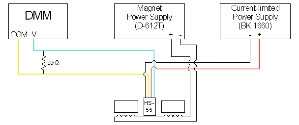
An overhead transparency of this schematic is available for you to display in class, or you may download a .pdf version here to show on the data projector.
When one places a current-carrying conductor in a magnetic field (perpendicular to the plane of the conductor), the charge carriers suffer a sideways force, F, equal to qvd × B, where q is the charge on each charge carrier, vd is the drift velocity of the charge carriers (given by j/ne, where j is the current density (in amperes/unit area cross section), n is the number of charge carriers per unit volume, and e is the charge per carrier; see demonstration 64.15 -- Resistance simulator) and B is the magnetic field (in Tesla). Since oppositely charged carriers have opposite drift velocities, for a given direction of current flow and magnetic field orientation, this sideways force is in the same direction regardless of the sign of the charge carriers (because the sign change for the charge and the sign change for the drift velocity cancel each other).
If we consider a pair of points x and y opposite each other at each edge of the strip, so that F pushes the charges from point x to point y, this sideways drift of charges produces a potential difference between x and y, the Hall potential difference, which we can denote Vxy. This is the potential difference that the voltmeter measures in this demonstration. The sign of the charge carriers determines the sign of Vxy. If the charge carriers are positive, y ends up at a higher potential than x; if they are negative, then y is at a lower potential than x. This potential difference also produces a transverse Hall electric field, EH = Vxy/d, where d is the width of the conductor (or the distance between x and y). This electric field opposes the sideways drift of the charge carriers until a point of equilibrium is reached where it just cancels the sideways magnetic deflecting force and qEH + qvd × B = 0, or EH = -vd × B. If we measure EH and B, we can find both the magnitude and direction of vd. If the direction is parallel to the current flow, the charge carriers are positive; if it is antiparallel to the current flow, the charge carriers are negative. These phenomena, and the effect in general, are named for Edwin H. Hall, who discovered them in 1879 American Journal of Mathematics, Vol. 2, No. 3 (Sep., 1879), pp. 287-292).
It is also possible to calculate the density of charge carriers by means of the Hall effect. When the drift velocity and the magnetic field are at right angles, their magnitudes and that of the Hall electric field are related by EH = vdB. If we substitute j/ne for vd, we get EH = (j/ne)B, or n = jB/eEH. We measure Vxy (or VH, as it is labeled in the photograph of the GaAs wafers), which equals EH/w, if we call the cross-wise dimension w. The area is wd, where d is the thickness of the layer. So VH = iB/ned, or n = iB/edVH.
This holds well for monovalent metals. The free-electron model on which the above analysis is based, however, fails for nonmonovalent metals, iron and similar magnetic materials, and for semiconductors such as germanium. (All the devices in this demonstration are semiconductors.) For such materials, one must use a quantum mechanical model to obtain an accurate calculation. Depending on the material and the doping level, however, one may be able to obtain a reasonable estimate.
References:
1) David Halliday and Robert Resnick. Physics, Part Two, Third Edition (New York: John Wiley and Sons, Inc., 1978), pp. 728-730.