Nuclear Magnetic Resonance Quantum Computing (NMRQC)
What is Quantum Computing?
Quantum Computing is a fundamentally new paradigm for information processing, harnessing the power of quantum mechanics.
How does it differ from classical
computation?
It differs from classical computation (your desktop) by being able to perform massive parallel computations.
What can we do with a quantum computer?
· Secure communication
· Search unsorted data bases faster than classical computers
· Factor integer numbers faster
· Simulating quantum mechanical systems efficiently.
1. Introduction to Classical
Information Theory
Let us quickly review some classical concepts of information theory. Information is real and physical and can thus be represented by physical systems: For example, in your computer, wires can be at 0 or 5 Volts with respect to some reference, representing the binary numbers 0 or 1. We can compute by taking many of these wires as inputs to some configuration of transistors, and in the end we measure the voltage on the output wires and translate it to an answer. This method of computing is very common but not unique! Note that your brain can multiply or add (small) numbers without paper and pen – Similarly, the abacus has been used extensively before our ‘electronic’ computers – or we could even use billiard balls! In fact, it does not matter how information is represented! If I were to give you a black box capable of computing, you would not be able to tell how exactly information is processed! This allows us to use the common notion of a Turing machine.
Furthermore, all information processing can be done reversibly. This is not obvious and not done in typical computers. Computers today consist of NAND gates (a fundamental building block for any logic circuit), which take two inputs and have one output. It is thus impossible to obtain the inputs just based on the outputs.
NAND-gate
|
Input |
Output |
|
00 |
1 |
|
01 |
1 |
|
10 |
1 |
|
11 |
0 |
Because of this, information is lost (or erased) which requires energy, which is the most fundamental reason why your desktop computer requires energy. Consider now the following gate – a doubly controlled NOT with 3 inputs and 3 outputs, where the 3rd input is set to ‘1’ so that the 3rd bit is flipped only if the 1st AND the 2nd are ‘1’:
CCNOT-gate (Toffoli)
|
Input |
Output |
|
001 |
001 |
|
011 |
011 |
|
101 |
101 |
|
111 |
110 |
So now, the 3rd bit equals the NAND of the 1st and 2nd bits. If we apply the same gate again, we retrieve the same numbers as in the ‘Input’ so that this gate is reversible. In fact, the NAND gate together with the NOT are universal gates, and we can build any logic circuit just based on these 2 gates. Since the Toffoli is reversible (and so is the NOT gate) we can build any logic circuit reversibly.
2. Introduction to Quantum Computing
Why is all of this important for
Quantum Computing?
First, since it doesn’t matter how information is represented, we could just as well go ahead and use a quantum mechanical system! Second, isolated quantum systems can ONLY evolve reversibly so it is important to be able to perform reversible computation.
Let us then take a two-level quantum mechanical system. This system can be in the state
![]()
The numbers ‘a’ and ‘b’ can be
complex numbers satisfying the normalization condition ![]() and the
and the ![]() is just quantum mechanical notation.
Consider the case where we only allow a=1 or b=1. This would be similar to the
classical regime because now the quantum bit (qubit)
is either ‘0’ or in ‘1’. Provided we can also perform NOT and Toffoli gates, we can build any classical logic circuit so
that a quantum computer can do everything a classical
computer can do. Of course this not the end of the story. Let us now
consider the case where
is just quantum mechanical notation.
Consider the case where we only allow a=1 or b=1. This would be similar to the
classical regime because now the quantum bit (qubit)
is either ‘0’ or in ‘1’. Provided we can also perform NOT and Toffoli gates, we can build any classical logic circuit so
that a quantum computer can do everything a classical
computer can do. Of course this not the end of the story. Let us now
consider the case where ![]() . This
is called a quantum mechanical superposition, and has absolutely no classical
analogue, but it is real and has been experimentally verified! It is as if the qubit is in ‘0’ and ‘1’ AT THE SAME
TIME. Suppose we take this state
as the input to some function f(x). The output would then be
. This
is called a quantum mechanical superposition, and has absolutely no classical
analogue, but it is real and has been experimentally verified! It is as if the qubit is in ‘0’ and ‘1’ AT THE SAME
TIME. Suppose we take this state
as the input to some function f(x). The output would then be ![]() , i.e.
a superposition of BOTH possible answers! Even though we though we only sent
, i.e.
a superposition of BOTH possible answers! Even though we though we only sent ![]() through f(x) once, we actually calculated 2
values. Now consider the case of 2 qubits with the
state:
through f(x) once, we actually calculated 2
values. Now consider the case of 2 qubits with the
state:
![]()
with ![]() .
Sending this state through f(x) only once calculates 4 values:
.
Sending this state through f(x) only once calculates 4 values:
![]()
In general, for ‘n’ qubits we can then write:

where  . So
then, for ‘n’ qubits, we can
perform up to 2n parallel computations! But how do we measure
all of the results? How do we obtain our answer to the computation? Suppose we
just measure the ‘n’ qubits. According to the laws of
Quantum Mechanics, the state
. So
then, for ‘n’ qubits, we can
perform up to 2n parallel computations! But how do we measure
all of the results? How do we obtain our answer to the computation? Suppose we
just measure the ‘n’ qubits. According to the laws of
Quantum Mechanics, the state ![]() will collapse to only one the 2n
states
will collapse to only one the 2n
states ![]() with probability
with probability ![]() (remember that a quantum mechanical
measurement is an irreversible operation). Thus we only get 1 answer, and in
general, we don’t even know which input this answer corresponded to. Thus, just
sending this parallel state through our function f(x) is not the correct way to
use the power of quantum mechanics. Instead, clever
algorithms have to be designed to achieve a speed-up compared with classical
computers.
(remember that a quantum mechanical
measurement is an irreversible operation). Thus we only get 1 answer, and in
general, we don’t even know which input this answer corresponded to. Thus, just
sending this parallel state through our function f(x) is not the correct way to
use the power of quantum mechanics. Instead, clever
algorithms have to be designed to achieve a speed-up compared with classical
computers.
3. Quantum Algorithms
To this stage there are 2 famous quantum algorithms, which allow a quantum computer to fundamentally perform certain tasks faster than any classical computer:
Shor’s Quantum Factoring
Algorithm
Grover’s Search Algorithm
Shor’s algorithm permits us to find the prime factors of l-digit integers in time proportional to only l3. The best known classical algorithm would take time proportional to (2l)(1/3) which is exponential in ‘l’. So for sufficiently large ‘l’ it becomes impossible to find the prime factors of numbers on even the best classical supercomputers. This ‘fact’ underlies most encryption codes used in secure communications today. Thus, a working quantum computer would defeat most encryption codes.
Grover’s Algorithm allows us to
search an unsorted database of size ‘N’ in time proportional to ![]() compared
with the classical case which would take time proportional to N. We will
explain how this algorithm works because it can be explained pictorially.
compared
with the classical case which would take time proportional to N. We will
explain how this algorithm works because it can be explained pictorially.
Consider the following scenario: Suppose you have ‘n’ bits and you have some complex logic circuit (x1 AND x2) OR (NOT x3 XOR x4) … etc. You know that the output of this function is TRUE only for one possible input, and you want to know which one it is. Classically, you would just proceed to look at each possible input until your output is ‘1’. On the average this takes N/2 attempts where N=2n. For example, suppose you have 2 bits and you wish to know for what values the function x1 AND x2 is TRUE. Classically, you would build the logic circuit that performs this operation. In this case it is just an AND gate. You would then go ahead and check the output for the all of the inputs, starting with ‘00’, until you get a ‘1’ as your output. If you did not get a ‘1’ as your answer by the time you get to ‘10’ you know that ‘11’ has to be correct (assuming there exist at least one solution). So it would take you 3 ‘queries’ to find the solution to your problem.
In general, for 2 bits, it would take 2.25 queries. Let us now use this 2 bit example to show how Grover’s Algorithm works. Let us initialize the 2 qubit quantum system to an equal superposition of all possible inputs:

Let us redraw the amplitudes of all the states in the following schematic:
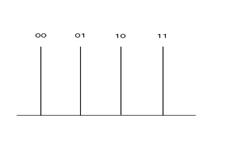
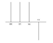
If we were to measure this state, then we would get ‘00’, ‘01’, ‘10’ and ‘11’ with equal probability (P=1/4). Let us now build an AND-like gate, which flips the amplitude of the state where (x1 AND x2). This circuit has no classical analogue (it is not meaningful to flip the phase of a DC voltage on a wire), and furthermore, we can build this circuit without knowledge of the outcome! Then, the amplitudes will look as follows:
In terms of measurement, nothing changed since the probability is the absolute value of the amplitude squared. However, suppose we can build some circuit that flips all of these amplitudes about their average values. The average value of the amplitudes is ¼. The ‘00’ state has an amplitude of ½. When we flip this about ¼ we get 0 amplitude! The same applies for all states except for the ‘11’ state, which gets amplified to ‘1’. So following this ‘inversion about average’, the systems looks as follows:
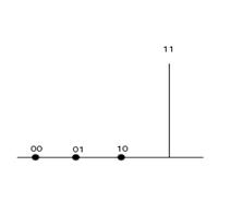
Now, if we measure we always get
‘11’ as our answer! Loosely speaking, the ‘phase flip’ and ‘inversion about
average’ is referred to as ‘querying’ the function f(x) once. So for 2 qubits, on the average we only need 1 function evaluation
compared with the classical case where we need 2.25 function calls!! For ‘n’ qubits we would need ![]() phase
flip and inversion about average steps compared to
phase
flip and inversion about average steps compared to ![]() function
calls classically.
function
calls classically.
Essentially, Grover’s algorithm relies on quantum interference effects to amplify the correct answer. Shor’s algorithm works in a very similar way but is too complicated to explain in detail here.
There are other applications of quantum computers, for example you could use a quantum computer to simulate some quantum mechanical system efficiently, which is not possible to do on a classical computer. The topic of quantum algorithms, and what can be done faster on a quantum computer is an active field of study.
One very important aspect ignored so far is error correction because real systems always have some error. So, in order to build a real quantum computer we need to be able to perform error correction! We will not go into detail here, but just state that error correction IS possible on a quantum!!
4. Basics of NMRQC
In order to build a quantum computer, we need to fulfill 6 criteria:
· A quantum system with qubits
· Individually addressable qubits
· Two qubit interactions (universal set of quantum gates)
· Long coherence times
· Initializing the quantum system to a known state.
· Extract the result from the quantum system.
Meeting all of these criteria simultaneously presents a significant experimental challenge. On the one hand, we want to system to be isolated from the environment so that coherence times are long (the coherence time is a measure for how long a quantum system can stay in a superposition). On the other hand, we need to address these qubits in order to perform a computation at all. This automatically requires coupling with the environment, causing decoherence. The challenge thus lies in finding a system which balances the opposing reuquirements.
NMR systems have been well studied for over 50 years now. The technology can be directly applied to quantum computing experiments. We will focus on liquid state solution NMR techniques.
1. A system of qubits: Nuclear magnetic Resonance Quantum Computers use the nuclear spin of atoms within a molecule as the quantum mechanical system. Specifically, we use spin-1/2 nuclei for this purpose. When such a spin is subjected a strong static magnetic field B0 (~200.000 times as strong as earth’s magnetic field) it can align or anti-align with this static field, similar to a classical bar magnet. We could label these two states as a logical 0 or 1. A spin precesses at a particular resonance frequency about this static field, much like a spinning top.
2. Individually addressable qubits: Each spin-1/2 can be individually addressed if it belongs to a different type of nucleus. For example, the signal from a spin-1/2 Hydrogen is at a very different frequency than the one from a Fluorine. If we have two Hydrogen but their chemical environment differs then they too can have different frequencies.
3. Universal set of quantum gates: Each spin-1/2 can be addressed by applying a radio-frequency pulse tuned to its resonance frequency. By timing the duration and phase of this pulse we can tip the spin into any direction. This allows us to implement single qubit gates. Two qubit gates require an interaction between qubits which is achieved by using the natural scalar coupling between the spins through shared electrons. We don’t require all spins to be coupled to each other. All we require is that there exists a network of couplings that connects the spins (for example a linear chain of spins with just nearest neighbor couplings is sufficient).
4. Long decoherence times: The cohrence times for spin-1/2 nuclei in NMR range from milli-seconds to seconds (and in special circumstances even minutes, hours or days). The time for a two-qubit gate can be on the order of milli-seconds. Thus we can expect to execute several tens, hundreds or thousands of operations using NMR
5. Initializing the quantum system to a known state: We perform all experiments at room temperature. But at that temperature the initial state is highly mixed. There are methods that allows us to transform the mixed state into an effective ‘pure’ known state but that requires exponential effort with increasing number of qubits. For the small number of qubits in our system we use these ineffective methods. There does exist one method that scales efficiently with increasing number of qubits but is impractical for current systems.
6. Extract the measurement from the quantum system: We measure the average signal from a sample containing about 1018 molecules using the same RF coils that produce the single qubit rotations.
How does this NMR Quantum Computer look like?

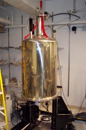
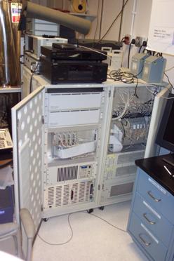
… more later.