Rupture growth, when considered from a dynamic point of view, is an elastic wave diffraction process. The reason for this lies in that way that the fault processes are specified mathematically as a mixed boundary value problem. This should be contrasted to the customary kinematic description of the earthquake source.

To be specific, what we would like to understand is the connection between what happens on the fault and the ground shaking we experience some distance away. Mathematically, we solve the elastodynamic wave equation off of the fault with some boundary conditions specified on the fault. In the customary kinematic description, this would amount to specifying the slip as a function of time at each point on the fault. Knowing this, we can easily determine how seismic waves transmit the shaking to distant regions of the earth. Such a description provides a linear relationship between ground displacements and fault slip, which can be exploited when solving the inverse problem (determining slip from recorded ground shaking). The main problem with this is that it precludes any mention of the forces acting on the fault.

Specifying the boundary conditions dynamically takes care of this problem. What we do is divide the fault into two regions, those ahead of the rupture front (crack edge) where the fault is locked and those behind, where we wish to prescribe the loss of strength accompanying material failure. In the second region, we switch from specifying slip to shear traction. Since the line along which these boundary conditions switch (the rupture front) moves with time, the problem becomes highly nonlinear, typically requiring numerical solution of the problem. The following figures explain this graphically.

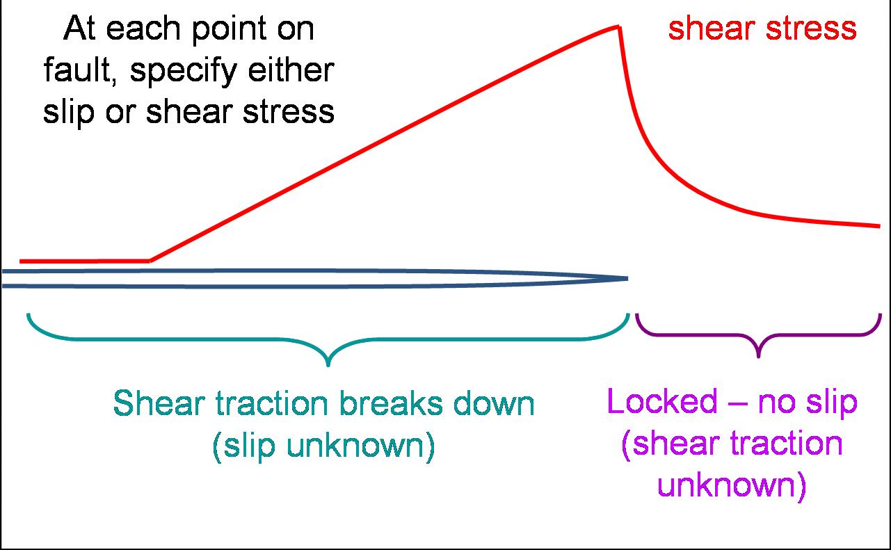
Figure 1: A 2D crack is shown in blue - imagine it moving to the right. The red line plots the shear stress on the fault. Notice that the stress rises from some constant value on the far right (corresponding to the initial tectonic loading) to a maximum at the crack tip. This value corresponds to the maximum strength of the frictional contact. To the left of this, the shear stress breaks down as the material fails and allows slip to relax the strain field. This occurs over some length scale, controlled by the time scale of the weakening process and the propagation velocity of the crack.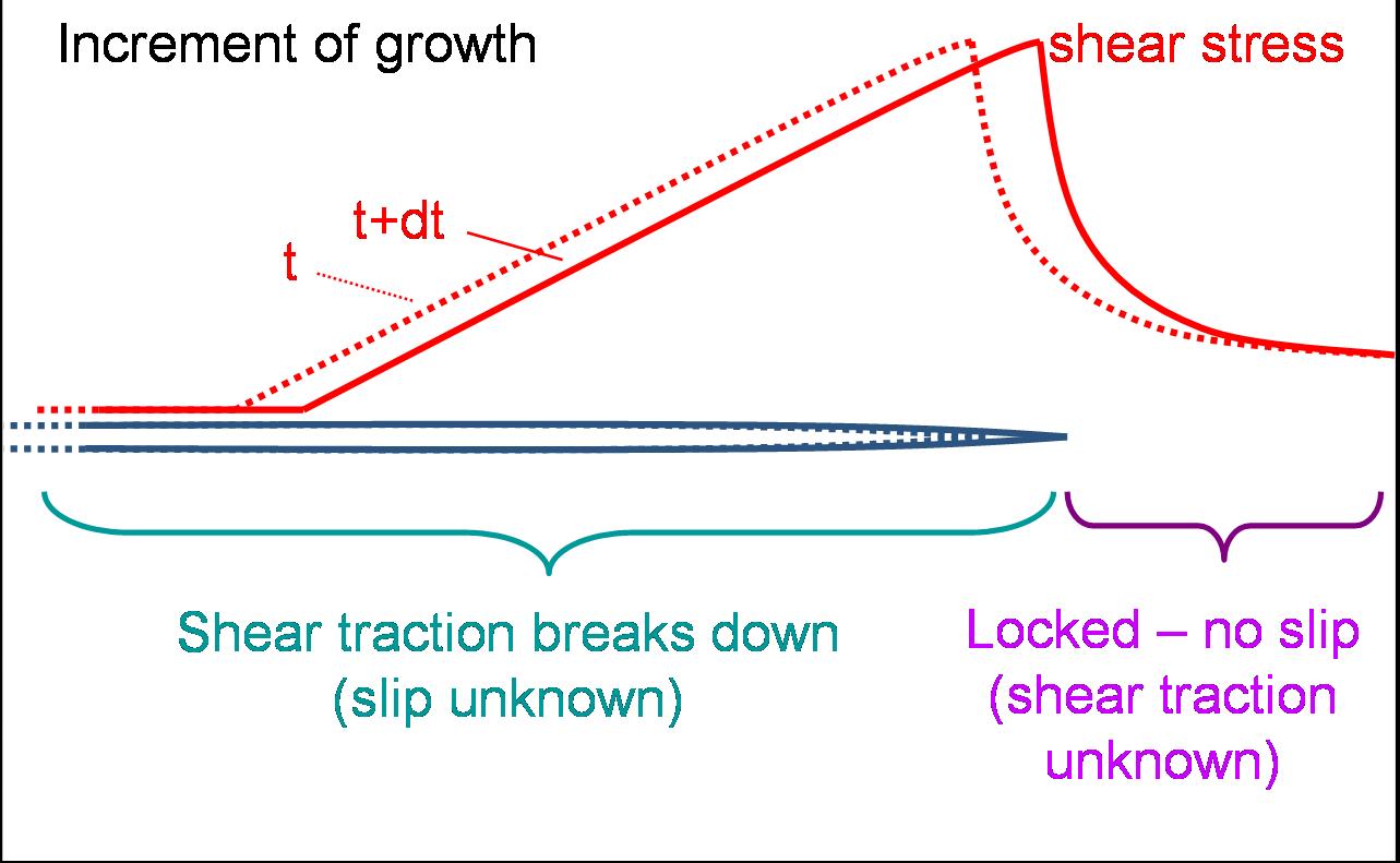

Figure 2: We now consider an increment of crack growth occuring over some short time dt. The crack advances to the right, and the shear stress breaks down behind the crack tip.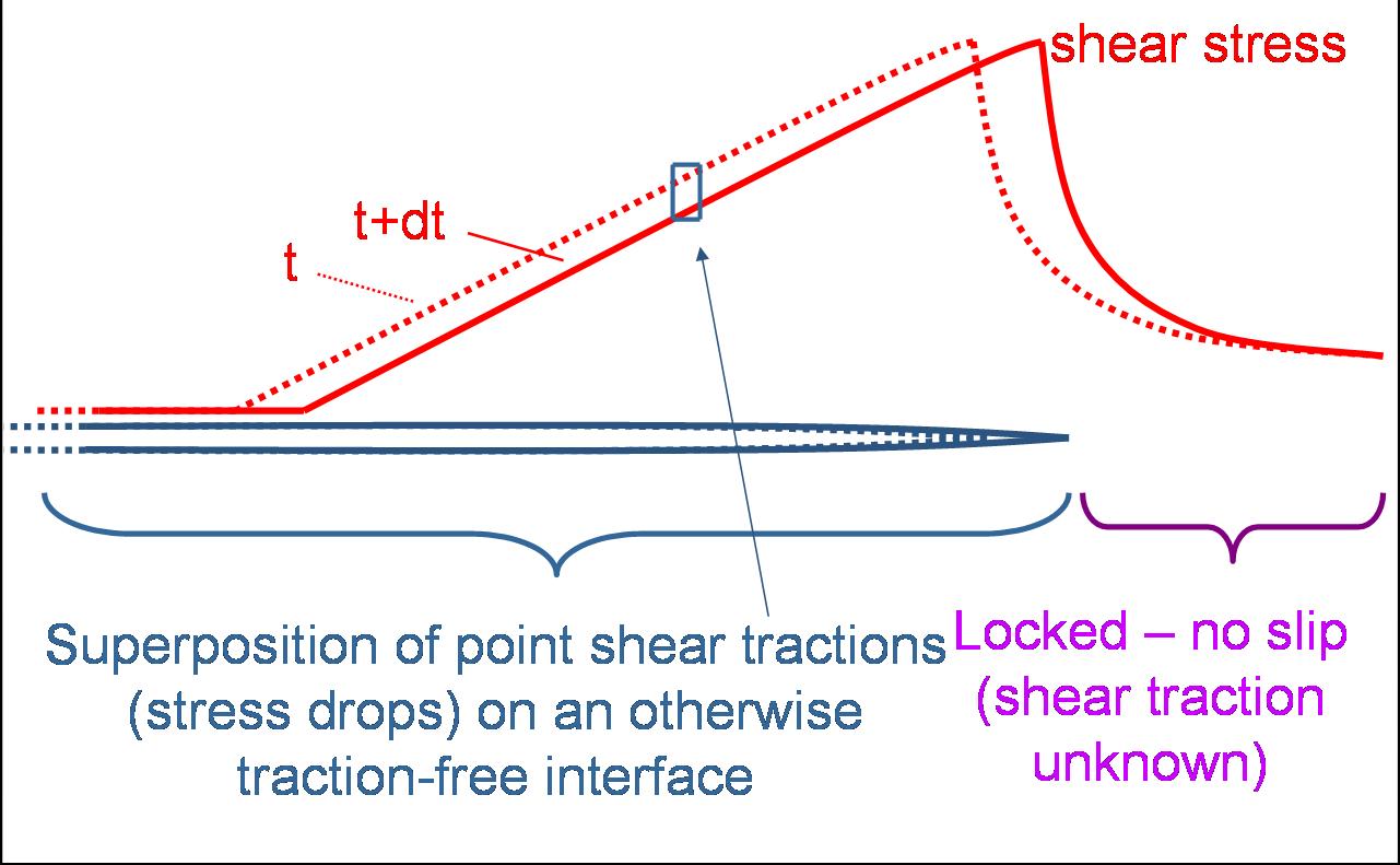

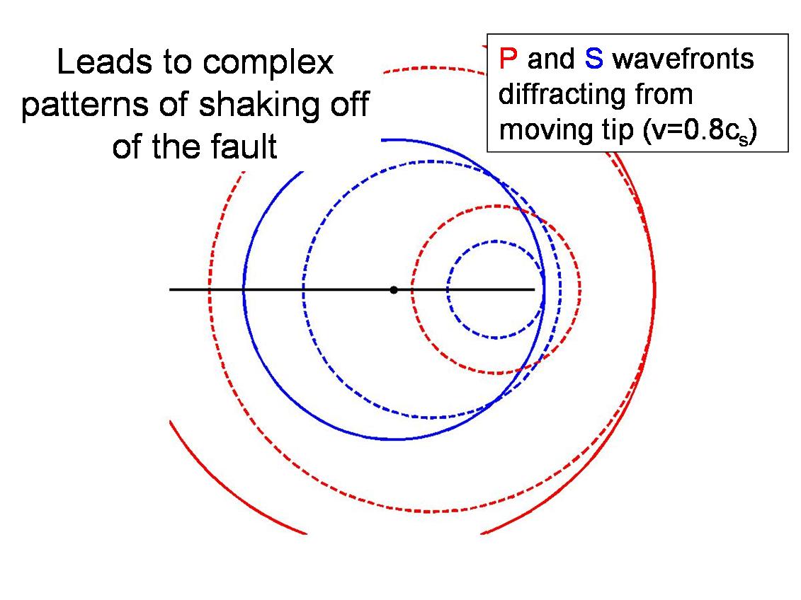
Figure 3: This is a boundary value problem. For boundary conditions, we specify that the fault is locked ahead of the (moving) crack tip - this requires knowledge of how it will move, and that the stress breaks down behind the crack tip. Since the elastodynamic equation is linear, we can use superposition to construct this breakdown in stress as a sum of stress drops applied some distance behind the crack tip, the remaining region behind the crack tip being traction-free.

The problem described above - a point stress drop some distance behind a moving crack edge - is a diffraction problem. The stress drop will release elastic waves that will overtake the moving crack edge and diffract off of it. An illustration is shown below. Note that these diagrams do not show all of the wave types, such as interface waves (Rayleigh waves) and head waves - both of which play an important role in rupture propagation. Further discussion of this problem and how it manifests itself in real earthquakes can be found in Dunham and Archuleta (submitted 2004 to BSSA)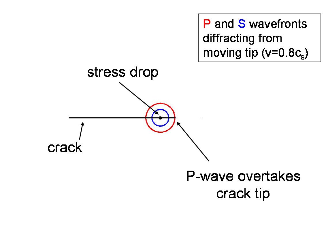

Questions? E-mail Eric Dunham