Radiation from Fault Heterogeneities

Radiation from Fault Heterogeneities

Barrier experiments of Dunham et al. [2003]

In a set of numerical experiments done by Dunham et al. [2003], it was found that in a three-dimensional medium, strong regions (barriers) can produce strong ground motion. In the figure to the left, rupture velocity is shown on the fault plane at successive steps in time. The rupture front hits a circular region of higher yield stress, which first stores energy as the rupture front surrounds it. As energy is focused inward, the barrier fails catastrophically, releasing a strong pulse of energy.

To investigate the ground motion produced by this complex dynamic process, we first construct a reduced barrier model with a constant rupture velocity. Using a 3D finite-difference method, we analyze the effect of barrier radius, strength, and depth, as well as the additional diffraction effects introduced by a time delay before the barrier breaks.

We follow the method of Andrews [1985] to solve the barrier problem given a constant rupture velocity. Unlike in a kinematic model, this does not constrain the slip-time function of points of the fault. Rather, it forces slip to be zero ahead of a rupture front moving at constant velocity. Frictional strength is no longer a function of slip as in a slip-weakening friction law. Instead, for each point it falls linearly with time until it reaches a constant value below the prestress, as shown in the figure. This method constrains the rupture velocity to be constant.

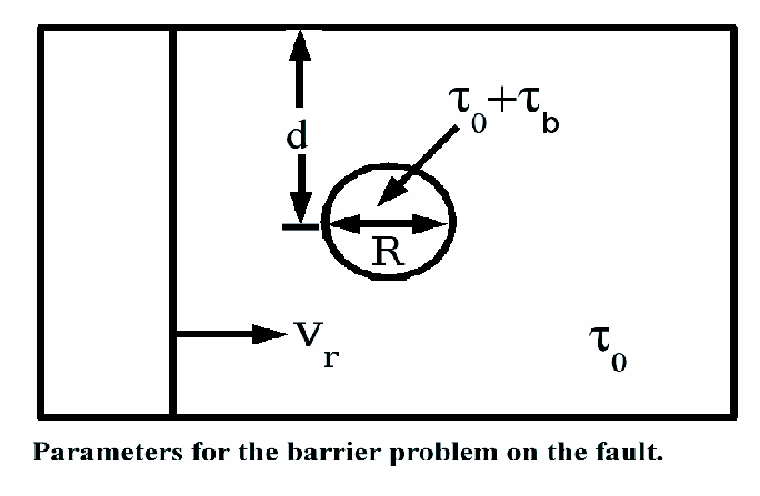We parameterize the barrier problem by R, the radius of the barrier, tau₀, the stress drop of the surrounding fault, tau_b, the additional stress drop in the barrier, and the depth d of the barrier.

For a small barrier, we expect the ground motion of our reduced model to be similar to the superposition of a homogeneous rupture and a point source, with the added effects of diffraction off of the crack edge. After subtracting off the displacements for a homogeneous rupture, this model cleanly shows that all components of additional displacement are proportional to R² and tau_b, for all points on the surface, at all times. The scaling relationship for depth is more complicated, but this parameter has the most influence directly above the hypocenter. In addition, as expected, this model shows that rise time for surface displacement is not a function of tau_b. 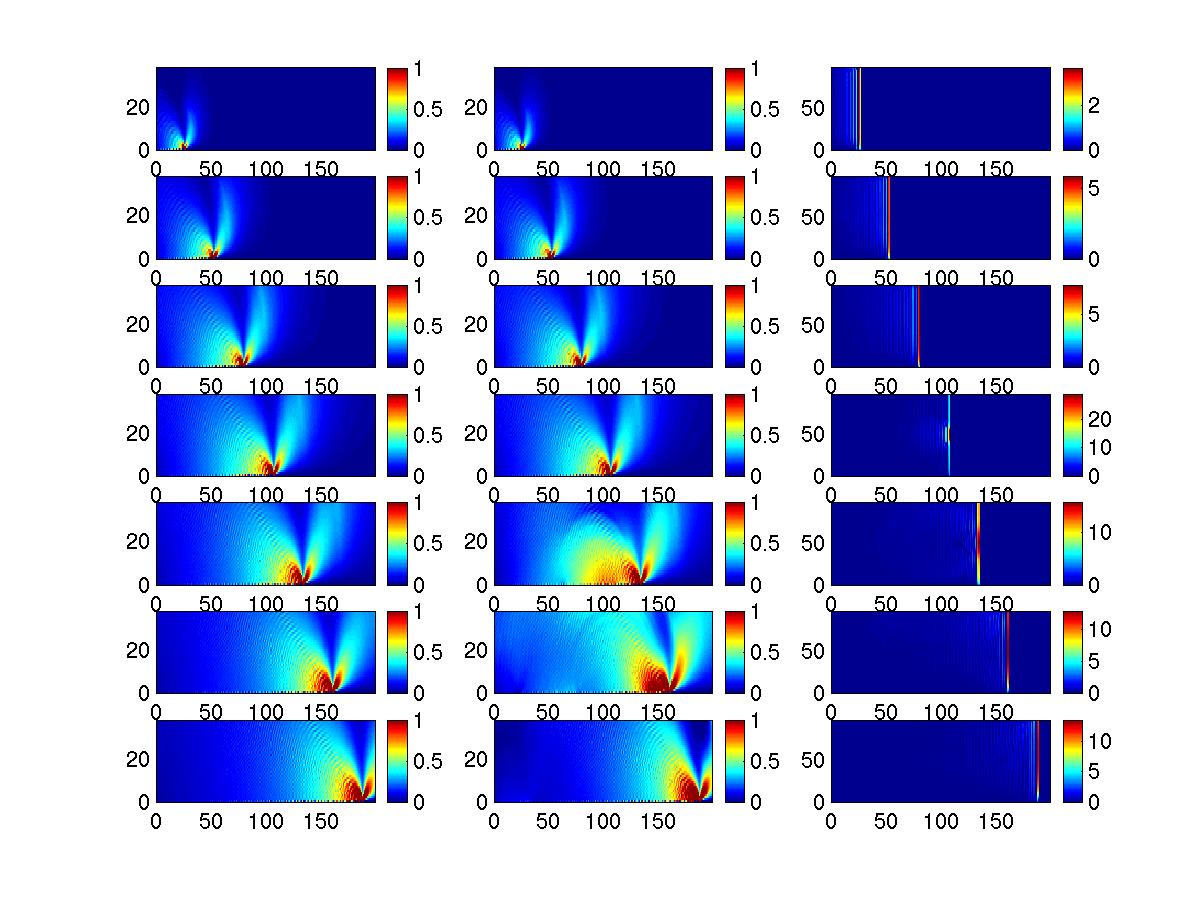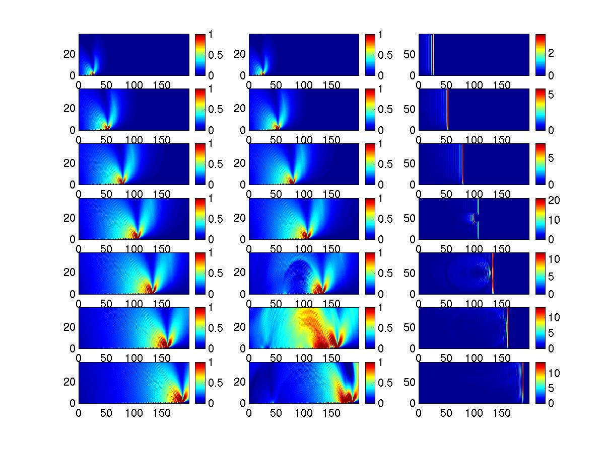Rise time for surface displacement increases with R and d, most notably in the forward direction from the barrier.

The first two columns of the figure on the right show fault-parallel displacements for the free surface for a homogeneous rupture (leftmost column) and the barrier rupture (middle column) at successive times. The bottom edge is the fault plane in these figures. The right-most column shows velocity on the fault plane for the barrier model.

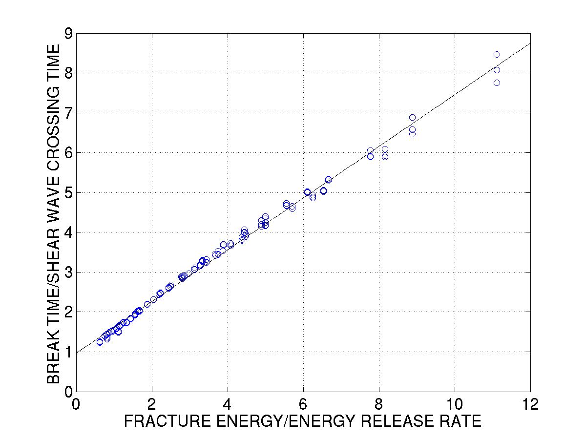
To make our model more realistic we next delay the breaking of the barrier by a time t_b. Numerical work by Dunham shows that this delay time is given by t_b=(2R/c_s)(1+aG/G₀), where R is the radius of the barrier, c_s is the shear wave speed, G is the fracture energy, and G₀ is the energy release rate. The constant a=0.6 was fit numerically using a slip-weakening friction law, as shown in the figure to the left.

This delay time makes the ground motion more dramatic: as the rupture front passes through the unbroken barrier, the stress increases, particularly at the edges of the unbroken region (see figure to right). When the barrier finally breaks, it breaks more violently than in the first model without the time delay.

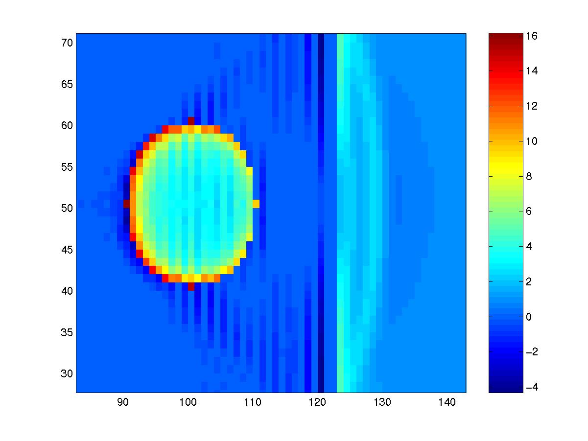Above: The stress increase in the locked barrier as the rupture front passes.

$Diffraction off Crack Edge$

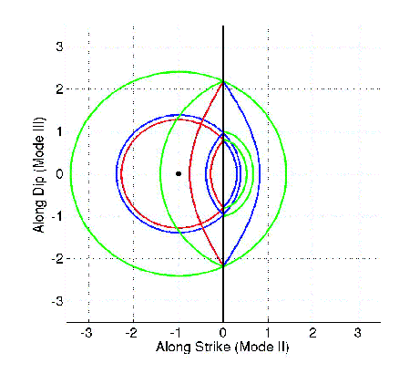
The barrier time delay also changes the diffraction effects from the first model -- for the crack edge is further ahead. The figure to the left shows the different wave fronts we can expect. The black circle shows the origin of a point source. The lines at the left side of the diagram show the velocity waves caused by the source: green curves are p-waves, blue are s-waves, and red are Rayleigh waves. To the right of the crack edge, the fault surface is unbroken, so that the curves shown are stress waves.

The middle column of the figure to the right shows the fault-parallel velocity at various times for our second model, with the barrier delay time. The last column shows velocity on the fault for the second model. Unlike in our original model, the barrier, initially locked as the rupture front passes, arrests the ground motion, before a larger pulse from the breaking of the barrier arrives.

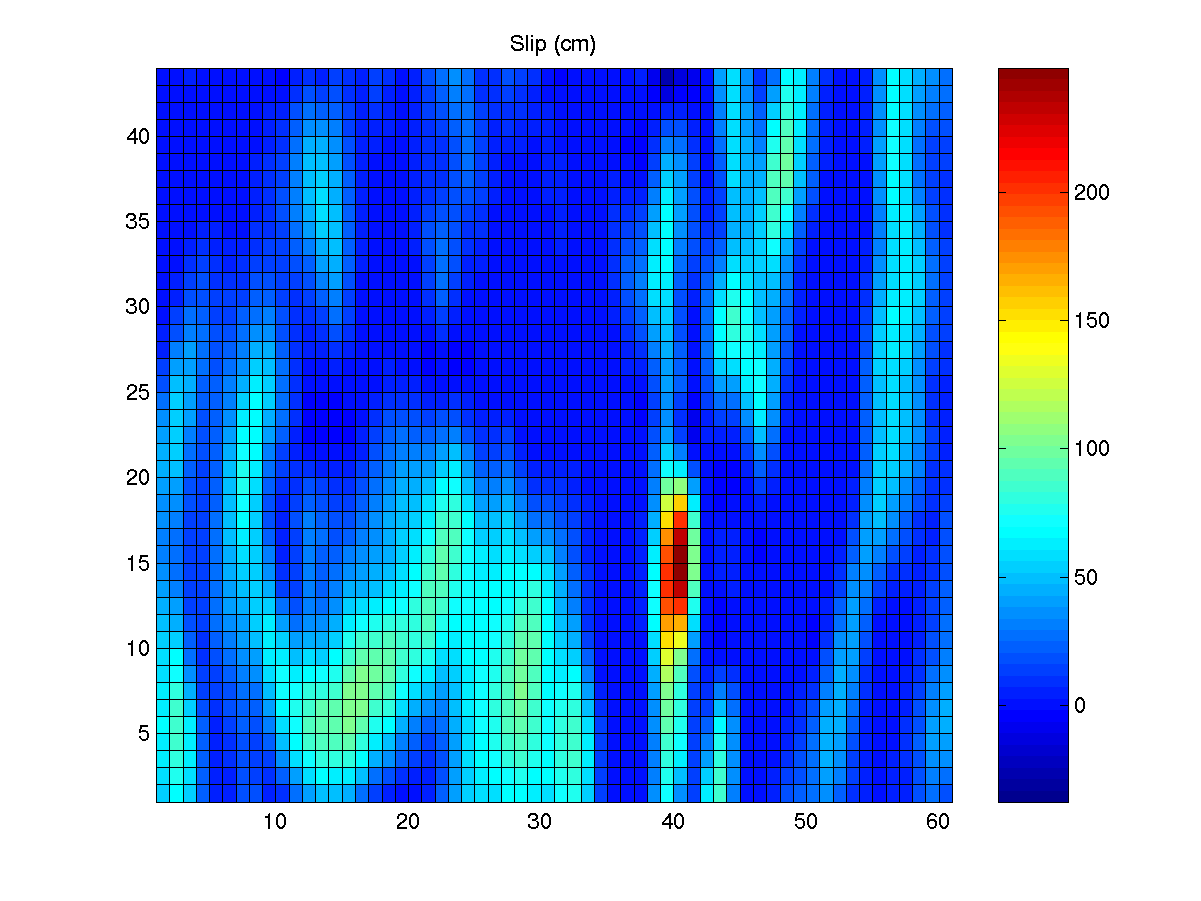
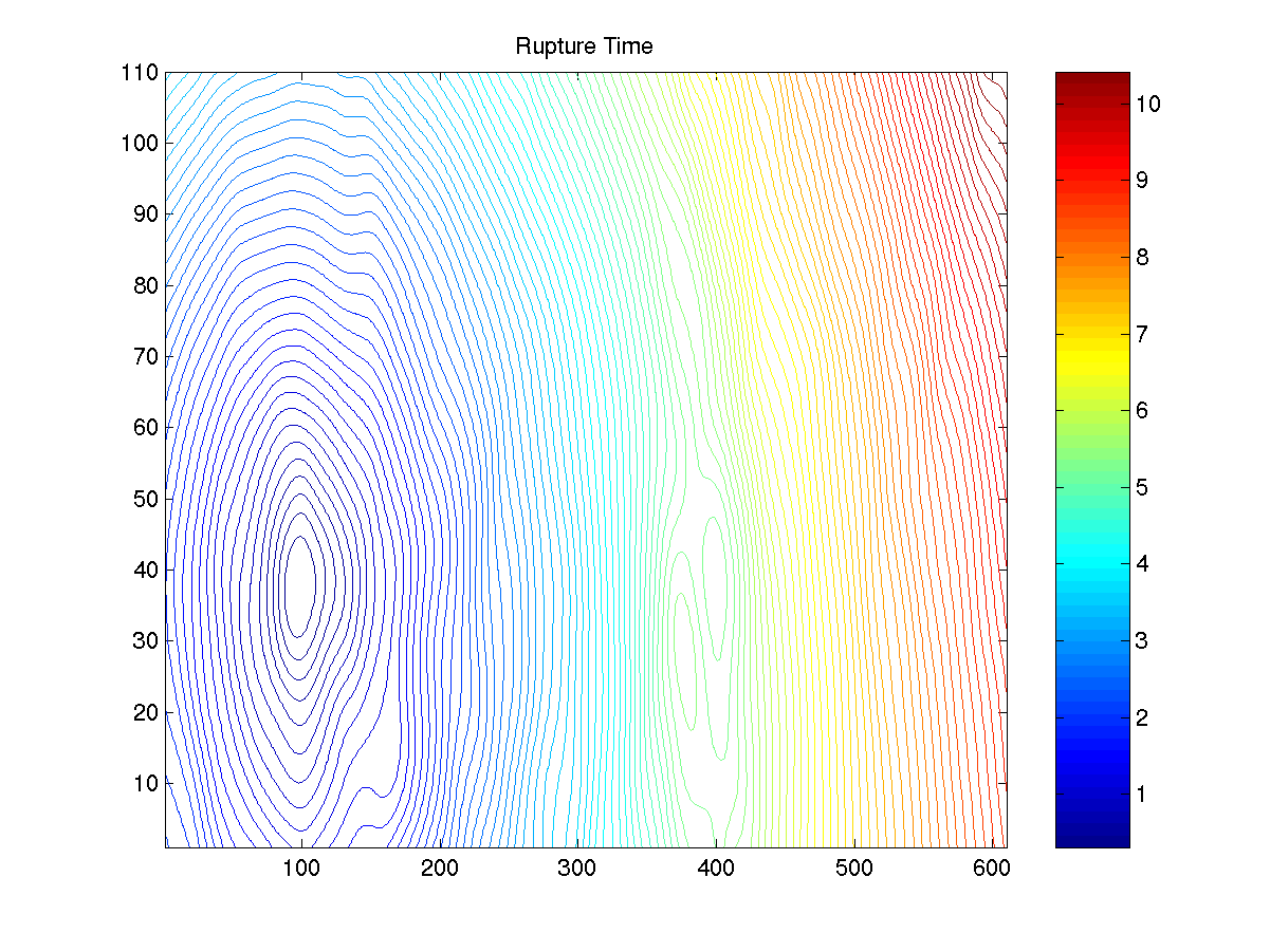
These models are not fully dynamic, as we are constraining the rupture velocity to be constant. The next step is to examine the fully dynamic problem, which may include supershear transients as seen by Dunham et al. The 1984 Morgan Hill earthquake may be a good example of an earthquake that can largely be characterized in terms of these barrier models.

The kinematic inversion of Beroza and Spudich [1988] shows that most of the slip in the Morgan Hill earthquake was concentrated in a small portion of the fault. The slip in this region is believed to be accountable for large, late pulses in several of the seismograms. Furthermore, their inversion shows a rupture delay in this region -- further evidence of a barrier. Finally, large fault parallel motions at the Coyote Lake Dam station may be evidence of supershear motion, as seen in the work of Dunham et al. [2003].

Above: The slip and rupture time on the fault for the 1984 Morgan Hill earthquake, as calculated in the kinematic inversion of Beroza and Spudich.

Questions? E-mail Morgan Page at:

References:

Andrews, D. J., Dynamic Plane-Strain Shear Rupture with a Slip-Weakening Friction Law Calculated by a Boundary Integral Method, BSSA, 75, 1-21, 1985.

Beroza, G. C., and P. Spudich, Linearized Inversion for Fault Rupture, J. Geophys. Res., 93, 6275-6296, 1988.

Dunham, E. M., P. Favreau, and J. M. Carlson, A Supershear Transition Mechanism for Cracks, Science, 299, 1557-1559, 2003.