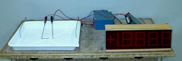
The blue power supply creates a potential difference between the two electrodes placed at the center of opposite edges of the pan of tap water. The two probes in the center of the pan are connected to the voltage input of the digital multimeter. By placing the probes in the water and moving them around, you can show the shapes of equipotential lines in various places. You can do this either by moving the probes so as to maintain a potential difference of zero between them, or by placing one of them very close to one of the fixed probes and moving the other so as to maintain a constant potential between them.

Electrically charged objects attract or repel other electrically charged objects, depending on whether the signs of their charge are opposite or the same, respectively. Demonstrations 56.03 – Attract paper bits with charged rod, and 56.06 – Electrostatically charged rods, show the action of these forces. The presence of such a force between charged objects indicates the presence of an electric field. At any point in this field, the magnitude and direction of the field are defined as the force a test charge would experience if it were placed at that point, or E = F/q, where q is the amount of charge on the test charge. The units of its magnitude are newtons/coulomb (N/C).

The shape of this field, that is, what its magnitude is at various points in the space around a charged object, depends on the shape of the object, the amount of charge on it, and the shapes of, and charges on, any other objects nearby. To help visualize electric (and magnetic) fields, Michael Faraday introduced the concept of lines of force. These are imaginary lines, which we draw such that the tangent of one at any point gives the direction of E there, and their density – the number of lines passing through unit cross-sectional area (perpendicular to the lines) – gives the magnitude of E. (The greater the density of lines, the greater the magnitude of E, and the fewer lines per unit area, the smaller the magnitude of E.) A line of force cannot begin or end in the space around a charge, but must begin at a charge and end at another of opposite sign. In the case of an isolated charge, we can think of the lines radiating from it as ending at many charges at great distance from the individual charge. Demonstration 56.27 Electric field patterns, illustrates how these lines look for a variety of electrode configurations. (The one that applies to this demonstration is the one that has two oppositely charged points.)

A test charge placed between two objects that have different quantities and/or signs of charge on them, is accelerated along a line of force that joins the two objects. Let us call the objects “A” and “B,” and say that the test charge is accelerated in the direction from A to B. A is thus at higher electrical potential than B, and in being accelerated toward B, the test charge gains kinetic energy equal to the potential energy difference through which it has traveled. This potential energy difference is the proportion of the potential difference between A and B that corresponds to the distance from B at which the charge starts in proportion to the distance between A and B. For example, if the potential difference between A and B is 10 volts, and the distance between them along the particular line of force is 10 cm, then if the charge starts at a point 2.5 cm from B, when it reaches B it will have acquired 2.5 volts of (kinetic) energy. For any given potential that lies between the potentials at A and B, there is a point on every line of force between A and B that is at that potential. The lines that connect the points on all the lines of force that are at the same potential are called equipotential lines. Since the lines of force extend in three dimensions, these equipotentials are actually equipotential surfaces. If, however, we take a plane that goes through both objects, we may examine the lines of force that lie within that plane, and the equipotential lines that are associated with them. These equipotential lines run perpendicular to the lines of force.

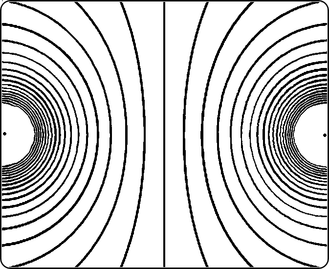
The apparatus in this demonstration consists of two point electrodes (the tips of two rods), one set at the middle of each end of a pan whose bottom is covered by a thin layer of tap water. The power supply puts a potential difference between the two electrodes. (This is usually set at 20 volts.) As noted above, the potential difference between the electrodes produces an electric field between them, associated with which are lines of force joining the two electrodes in a pattern similar to that shown for the two oppositely charged points in demonstration 56.27. A set of equipotential lines, which run perpendicular to the lines of force, is shown below.

As noted above, you can trace these equipotential lines in either of two ways. If you place the two probes on an equipotential line, the voltmeter reads zero. If you move one or both of the probes along the equipotential line, the reading remains zero. Thus, by manipulating the probes so as to keep the meter reading at zero, you can trace various equipotential lines. Alternatively, you can set one probe at one of the electrodes, and move the other probe in such a way as to keep the voltage between the probes constant. For example, with the power supply set at 20 volts, if you place one probe at the negative electrode and move the other probe along the vertical line at the center of the tray, the meter should show a constant reading of 10 volts.