A steel wire runs from an anchor at the left end of this apparatus, over two bridges, to a lever at right, by which you can apply tension to it. You can adjust the bridges to set the length of the vibrating portion of the wire. As shown in the photograph above, they are set 0.500 meters apart. The signal generator feeds a driver coil, in the small black box near the bridge at left, by which you can set the wire vibrating. A detector coil converts the vibrations of the wire into an electrical signal, which you can see on the oscilloscope. For a wire of given linear density (of which you have five choices), and a given tension, you can find the frequencies for the various harmonics of the wire, and show the patterns of the standing waves you form (vide infra). You can vary the tension to show how this affects the frequencies of the harmonics, and you can change the length of the vibrating part of the wire by moving either bridge, or both, as you wish.
The apparatus in the photograph above is a monochord, that is, an instrument that has a single string whose vibrating length and tension you can vary. If you pluck the string, it sounds a certain pitch, which depends on the vibrating length, tension and linear density (mass per unit length) of the string. Monochords date to ancient times. Perhaps the most famous experiments performed with a monochord are those by Pythagoras. His monochord had a moveable bridge, which divided the string into two sections. He found that if he placed the bridge so that the lengths of the two sections were in whole number ratios, the two pitches they produced sounded pleasing; they formed some musical interval. Probably because it allows one to study the physics of a vibrating string by observing the sound it produces, it is common for people to refer to such an instrument as a sonometer.
This particular sonometer is equipped with a driving coil, which when fed by a function generator and placed underneath the (steel) wire, causes the wire to vibrate, and a magnetic sensing coil, which converts the vibrations of the string into an electrical signal. The driving coil is essentially an electromagnet. When current flows through it, this sets up a magnetic field, which polarizes the part of the string sitting above it. This produces an attractive force, which displaces the string. Sending a periodic current through the coil thus sets the wire vibrating. The sensing coil has a slightly magnetized core, which polarizes the wire above it. Because the wire is thus magnetized, if it begins to vibrate, this causes a changing magnetic flux in the sensing coil, which induces an emf in it, causing a current to flow. (The polarization of the string is not great enough to displace it significantly. If it were, however, since the magnetic field is static, the displacement would be constant, and the wire should not vibrate.) When you drive the wire with a sine wave applied to the driving coil, if the driving frequency matches that of a harmonic of the wire, the wire begins to vibrate with significant amplitude (a phenomenon called resonance), and if you place the sensing coil under an antinode, you observe a sinusoidal trace on the oscilloscope.
Available with this apparatus are 10 wires, two of each of five diameters. These are:
Diameter
Linear Density
0.010″
0.39 g/m
0.014″
0.78 g/m
0.017″
1.12 g/m
0.020″
1.59 g/m
0.022″
1.84 g/m
Each wire has a cylindrical anchor at one end, and an eye at the other. The cylindrical anchor sits in the notch in the top part of the lever at the right end of the apparatus, and the wire goes through the slot in the lever. The eye at the other end of the wire goes on the pin on top of the cylindrical aluminum piece at the left end of the apparatus. By means of the knurled screw at left, adjust the position of this end of the wire so that the long part of the lever at right is level. There are five notches on the horizontal part of the lever. If you hang a mass m from the notch closest to the pivot, this produces a tension of mg in the wire. Hanging the mass from the second, third, fourth and fifth notches from the pivot gives tensions of 2mg, 3mg, 4mg and 5mg, respectively. Note the warning on the side of the sonometer base, which stipulates a maximum load of 1.75 kg on the lever.
As shown on the page for demonstration 40.54 – Waves on cord, tubing, spring, the velocity of a wave on a linear elastic medium such as a wire is
v = √(T/μ)
where T is the tension in the wire, and μ is the linear density of the wire. For a wave traveling in a medium, its velocity, frequency and wavelength are related by
v = νλ, so ν = (1/λ)√(T/μ)
Since a standing wave occurs any time an integral number of half wavelengths fits within the vibrating length of wire, L, we have
λ = 2L/n, and ν = (n/2L)√(T/μ)
At any frequency that satisfies this equation for a given value of n, we obtain a standing wave that has one node at each end of the vibrating length of wire, and n antinodes and n - 1 nodes between the ends. For the first harmonic, or fundamental, n = 1. If we call the frequency of the fundamental ν0, then we expect harmonics at frequencies of ν0, 2ν0, 3ν0, 4ν0, 5ν0, etc.
In the photograph above, the wire installed in the sonometer has a diameter of 0.017″, and the hanging mass is 1.05 kg. Hanging from the fourth notch, this mass exerts a tension of 4(1.05 kg)(9.81 m/s2) = 41.2 N. L equals 0.50 m, and the linear density of the wire is 1.12 × 10⁻³ kg/m. Putting these into the equation above gives a frequency of 192 Hz for the fundamental (n = 1).
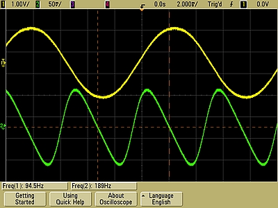
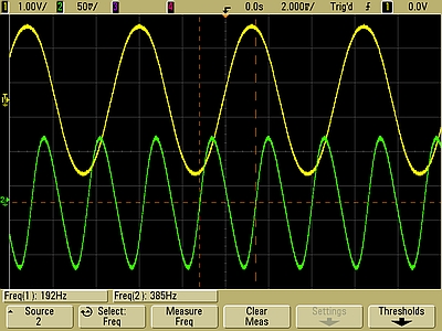
Because the magnetic field produced by the driving coil has a maximum every half cycle, it drives the wire at twice the frequency of the sine wave that feeds it. Thus, each harmonic you find with the detector coil occurs at twice the frequency of the sine wave with which you drive the wire. The images below show the wire being driven at the first two harmonics.
Fundamental
Second Harmonic
In each panel above, the top trace (channel 1, yellow) is the output from the function generator, and the bottom trace (channel 2, green) is the signal from the detector coil. For the traces in the left panel, the function generator is set to 94 Hz, and it excites the fundamental at 189 Hz, which is close to the frequency of 192 Hz calculated above. For panel at right, the function generator is set at 192 Hz, and it excites the second harmonic at 385 Hz. From these two traces, we can also see the 90-degree lag between the driving signal and the oscillation of the wire. (Remember that each half cycle of the driving wave corresponds to a full cycle of the driven wave. See demonstration 40.42 – Driven pendulums.)
You can slide the detector coil to different places, to show the locations of nodes and antinodes, and you can slide the driver coil to where it excites the string well, but does not interfere with the detector coil. When you first turn on the function generator, if it is not tuned near a harmonic of the wire, you probably will not hear anything. As you tune the function generator, when you approach a harmonic, the vibration of the wire will be great enough that you will hear the sound that it produces.
As the equations above show, increasing the tension on the wire raises the frequencies at which it vibrates, increasing the linear density of the wire lowers the frequency at which it vibrates, and increasing the distance between the two bridges lowers the frequency at which the wire vibrates.
The Overtone Series
The experiments of Pythagoras and others with monochords (and, most likely, also pipes), revealed to them what we now call the overtone series, which has tremendous significance to music. It provides the basis for musical scales and intervals. The overtone series is, of course, the harmonic series, but with a slight difference in nomenclature. In both series, the lowest-frequency member is the fundamental. It is common to refer to the second harmonic as the first overtone, the third harmonic as the second overtone, etc. As noted on the page for demonstration 44.12 – Ear model, we hear differences between pitches according to the ratios of their frequencies. That is, we hear any pair of pitches whose frequencies are in a particular ratio, as being the same musical interval apart. As noted above, the harmonics are successive integer multiples of the frequency of the fundamental. The interval between any two members of a harmonic series – two pitches whose frequencies are in whole number ratios – will sound pleasant. If the frequencies of two pitches cannot be expressed as a whole-number ratio, then the pitches are not harmonically related, and their interval sounds out of tune. As we go up in the harmonic series, the frequency ratios of neighboring harmonics become successively smaller, and thus, so do the musical intervals between them. A frequency ratio of 2:1, which we have between the second harmonic and the fundamental, corresponds to a musical interval of an octave. For the first three octaves in the harmonic series, the frequencies and intervals are as in the following table.
n ν Interval from Previous Harmonic Interval from Fundamental 1 ν0 Unison (perfect prime)
Unison (perfect prime)
2 2ν0 Octave Octave 3 3ν0 Perfect fifth Octave + One perfect fifth 4 4ν0 Perfect fourth Two octaves 5 5ν0 Major third Two octaves + One major third 6 6ν0 Minor third Two octaves + One perfect fifth 7 7ν0 Minor third* Two octaves + One minor seventh* 8 8ν0 Major second* Three octaves Intervals are named according to the number of scale degrees that separate the two pitches that make them. Going up from the first step of a major scale, the tonic, the rest of the scale steps are, in succession, a major second, major third, perfect fourth, perfect fifth, major sixth, major seventh and an octave above the tonic. The intervals between neighboring scale degrees are major and minor seconds – whole steps and half steps, respectively.Within the first three octaves of the harmonic series, we have the major third, which corresponds to a frequecy ratio of 5:4, the perfect fourth, whose ratio is 4:3, the perfect fifth, whose ratio is 3:2, and the octave, at 2:1. The asterisks on the intervals for the seventh and eighth harmonics are there because though they are close, they do not equal the ratios by which we normally define these intervals. The building of scales and intervals from the overtone series is a rich and fascinating subject. Suffice it to say here, that frequency ratios for the various intervals are commonly based on just intonation, a system in which all intervals are derived from the natural fifth, natural major third and natural octave, i.e., those shown in the table above. This system is considered to provide the most pleasant-sounding major triads (built on the first, fourth and fifth steps of the scale), because it puts them all in 4:5:6 ratios. (Note that the fourth, fifth and sixth harmonics together make up a major triad. This property is probably why the German name for just intonation is reine or natürliche Stimmung, for “pure” or “natural voicing.”) Unfortunately, this system has serious disadvantages that prevent its use for tuning instruments, but it does provide a useful reference for calculating frequency ratios for intervals that we hear as being “pure” or “natural.” Intervals having these frequency ratios are called just-tuned or just. The ratios given above for the major third (5:4), perfect fourth (4:3), perfect fifth (3:2) and octave (2:1) correspond to those for just-tuned intervals. A just minor second has a frequency ratio of 16:15, major second 9:8, minor third 6:5, minor sixth 8:5, major sixth 5:3, minor seventh 16:9, and major seventh 15:8.
References:
1) Resnick, Robert and Halliday, David. Physics, Part One, Third Edition (New York: John Wiley and Sons, 1977), pp. 412-413.
2) Berg, Richard E. and Stork, David G. The Physics of Sound (Englewood Cliffs, New Jersey: Prentice-Hall, Inc., 1982), pp. 67-75, 319-320, 349-351.
3) Apel, Willi. Harvard Dictionary of Music (Cambridge, Massachusetts: Harvard University Press, 1955) pp. 359-363 (Intervals, and Intervals, Calculation of), pp. 384-385 (Just intonation).