The square wave output of a signal generator is connected to a variable resistor and a capacitor in series. The voltages across the pair (top trace), the capacitor (middle trace) and the variable resistor (bottom trace) are shown on the oscilloscope, whose display you can project to the class via the data projector.
Demonstration 64.51 -- RC to galvanometer(s) shows the charging of a capacitor through a resistor. Once a capacitor is so charged, if we short the opposite ends of the capacitor and the resistor together so that they now form a loop, the capacitor discharges through the resistor. (In demonstration 64.51, you can show this by shorting the free end of the resistor to common, either through the ammeter or not, as you wish.) One way to perform the same thing, that is, alternately to charge and then to discharge a capacitor through a resistor, is to apply a square wave potential. During the positive portion of the square wave, a voltage is applied across the resistor-capacitor pair, and the capacitor charges. During the zero portion of the square wave, the potential across the resistor-capacitor pair is zero, as it would be if we had a switch to short the two ends together, and the capacitor discharges. Whereas demonstration 64.41 has four different-size capacitors, each connected to a 1-k resistor, in this demonstration a 0.01-μF capacitor is connected in series with a 100-k variable resistor. To provide an appropriate time scale for viewing the charge and discharge cycles of the capacitor, the function generator is set to a frequency of 1 kHz.
If we call the potential applied by the function generator during the positive half cycle VApp, then VApp = VR + VC = iR + q/C. The current, i, is dq/dt, and we have VApp = R(dq/dt) + q/C. The solution to this differential equation is q = CVApp(1 - e-t/RC). Since the voltage across the capacitor is q/C, we can also write this as VC = VApp(1 - e-t/RC), which gives us the voltage across the capacitor as a function of time. During the half cycle when the square wave is zero, VApp is zero, and VR + VC = 0 = iR + q/C, or 0 = R(dq/dt) + q/C. For this equation the solution is q = q0e-t/RC, where q0 is the charge on the capacitor at the beginning of the half cycle, and equals V0C, where V0 is the voltage across the capacitor at the beginning of the half cycle. (In other words, the voltage to which it had charged by the end of the previous half cycle.) So the voltage across the capacitor during this half cycle is V = V0e-t/RC.
In the equations above, the product in the denominator of the exponent, RC, is called the time constant, and is often denoted as τ. This is the time it takes for the voltage across the capacitor to reach 63% of the applied voltage during the positive half cycle, or 37% during the zero half cycle. (At t = RC, the term in parentheses in the equation that describes the positive half cycle equals 1 - e-1, or 1 - 0.37 = 0.63. The equation for the zero half cycle contains only the exponential term, which equals 0.37.)
To find the current for each half cycle, we can either differentiate the equations above for q to get dq/dt = i, or we can note that VR = iR, and arrange the equations above in terms of VR. Either way, this gives for both half cycles i = (VR/R)e-t/RC. For the charge cycle (the positive half cycle), V starts at the value of the applied voltage, and as the capacitor charges, it diminishes to zero. Since the capacitor is charging, current is flowing into it, and the current is positive. During the discharge cycle (the zero half cycle), the capacitor is discharging, so current is flowing out of it, and the current is negative. VR starts at whatever VC was at the end of the positive half cycle, and diminishes to zero. (Since VR + VC = 0 for this cycle, VR = -VC.)
In the discussion above, we assume that the half cycles are sufficiently long compared to the RC time constant that the capacitor can charge to the point where VC ≈ VApp, and discharge until VC ≈ 0.
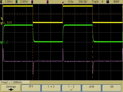
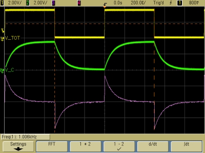
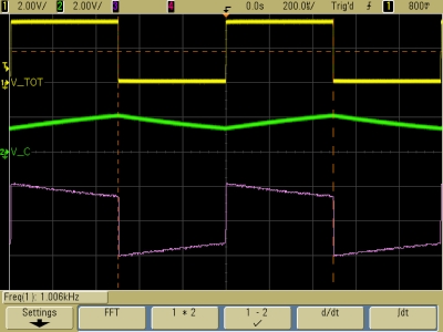
Below are three examples of oscilloscope traces for this demonstration:
τ ≈ 8 μs (R ≈ 800 Ω)
τ ≈ 80 μs (R ≈ 8,000 Ω)
τ ≈ 1,000 μs (R ≈ 100 kΩ)
In each of the displays above, the top trace is the voltage applied by the function generator (V_TOT), the middle trace is the voltage across the capacitor (V_C), and the bottom trace (unlabeled) is the voltage across the resistor (the difference between V_TOT and V_C), which is directly proportional to the current. The horizontal scale is 200 μs per division, and the frequency is about 1 kHz (so 1,000 μs per cycle). For the left-hand display, the RC time constant, τ, is probably around 8 μs, so R is set to about 800 ohms. In the middle display, τ is much larger – approximately 80 μs – so R is about 8,000 ohms. In the display at right, τ is relatively large – probably around 1,000 μs – so R is probably 100 k.
From these traces, we see that as τ approaches zero, VC begins to resemble the input square wave and VR → 0, and that as τ becomes large compared to the length of the half cycles, VC approaches the average of the voltages for the two half cycles, and VR begins to resemble the input square wave, shifted so that it is symmetrical about zero. (At the changes between half cycles, the capacitor begins to charge or to discharge from whatever voltage was across it at the end of the previous half cycle. As τ becomes larger and larger, the voltage across the capacitor approaches the average of the voltages for the two half cycles. If we subtract this average from the applied voltage, we get half the voltage for the positive half cycle, and minus the average voltage for the zero half cycle.)
References:
1) David Halliday and Robert Resnick. Physics, Part Two, Third Edition (New York: John Wiley and Sons, Inc., 1978), pp. 705-709.
2) Howard V. Malmstadt, Christie G. Enke and Stanley R. Crouch. Electronics and Instrumentation for Scientists (Menlo Park, California: The Benjamin Cummings Publishing Company, Inc., 1981), pp. 143-145.