Dynamic rupture
An earthquake can be viewed as either an instability in frictional contact or the growth of a shear crack. We model the crust of the earth as an elastic solid that can support an interesting variety of wave motions as well as static stress and deformation fields. Within this crust are fault planes, zones of weakness along which previous earthquakes have occurred. Due to the large scale tectonic motion of plates, large stresses accumulate within the ground. For example, here in Southern California, the Pacific and North American plate slide past each other along the San Andreas fault (you can imagine the fault as a vertical plane of contact extending from the surface down to about 10 or 15 km – see Figure 1). Below this depth, the increased temperature and pressure allow the rocks to move in a ductile manner that prevents the build-up of large stresses. But closer to the surface, the rocks are brittle solids that are being compressed by the enormous weight of the overlying rocks (something you might be familiar with if you've been buried in the sand at the beach!). This compressional stress will prevent the two sides of the earth from opening (which is what happens in a tensional crack). Since the two sides of the fault are always in contact, there will be a frictional force between them.
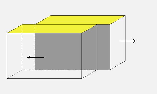
Figure 1: A fault, shown in gray, is a roughly planar zone of weakness in the crust. Tectonic motions of the earth’s plates drive the two sides of the fault past one another, represented here by the arrows. The yellow surface denotes the earth’s surface.
Now imagine trying to force the two sides to slide past each other. For the San Andreas, the western Pacific plate (on which Santa Barbara sits) is moving northwest relative to the eastern North American plate (on which most of the country sits) at a rate of about 30-40 mm/yr. This motion increases the shear stress on the fault over the course of decades or centuries, during which the fault is still locked (see Figure 2).
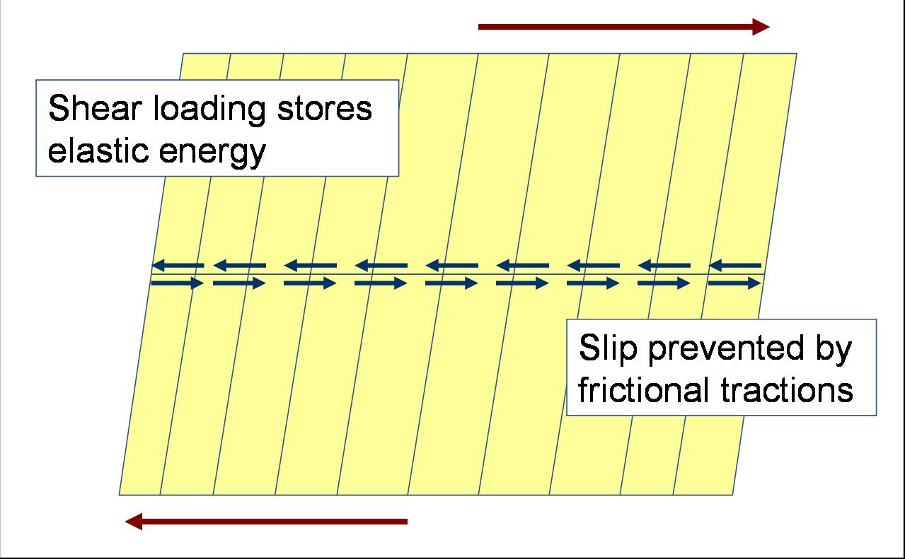
Figure 2: Top view of the geometry shown in Figure 1. The fault is the horizontal line through the center, with the blue arrows representing frictional forces that keep the sides of the fault locked. The slanted vertical lines indicate the shear displacements created by tectonic loading.
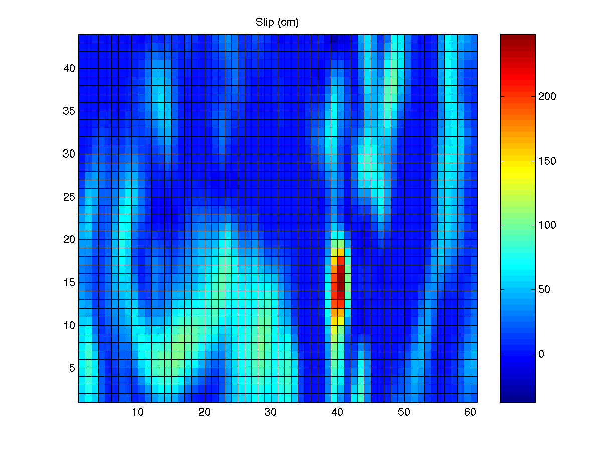
At some critical level, the force on the fault will exceed the static frictional force, and the two sides will start to slide with some dynamic frictional resistance (less than the frictional value). From a fracture point of view, there is a cohesive force that exists between the two sides of the fault, and the stress must be large enough to overcome this. The discontinuity in the relative displacement is called slip. When this process occurs rapidly, it converts some part of the released strain energy into seismic waves (see Figure 3).
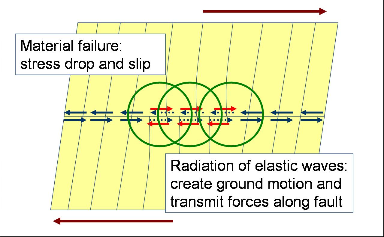
Figure 3: Material in the fault zone fails (or static friction is exceeded) and the fault begins to slip. Physically, we can view this process as the application of shear forces on the fault that negate the static friction, as represented by the red arrows. This releases elastic waves, indicated by the expanding green circles.
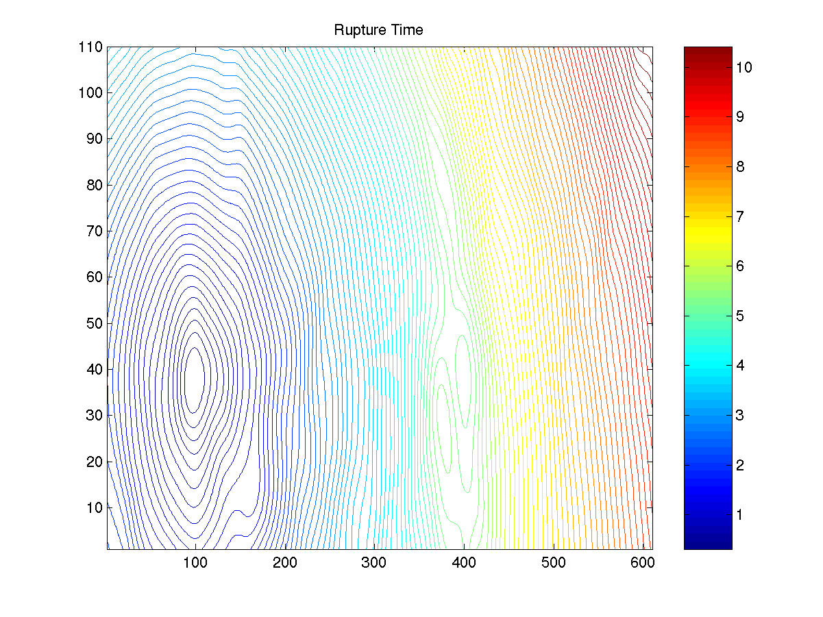
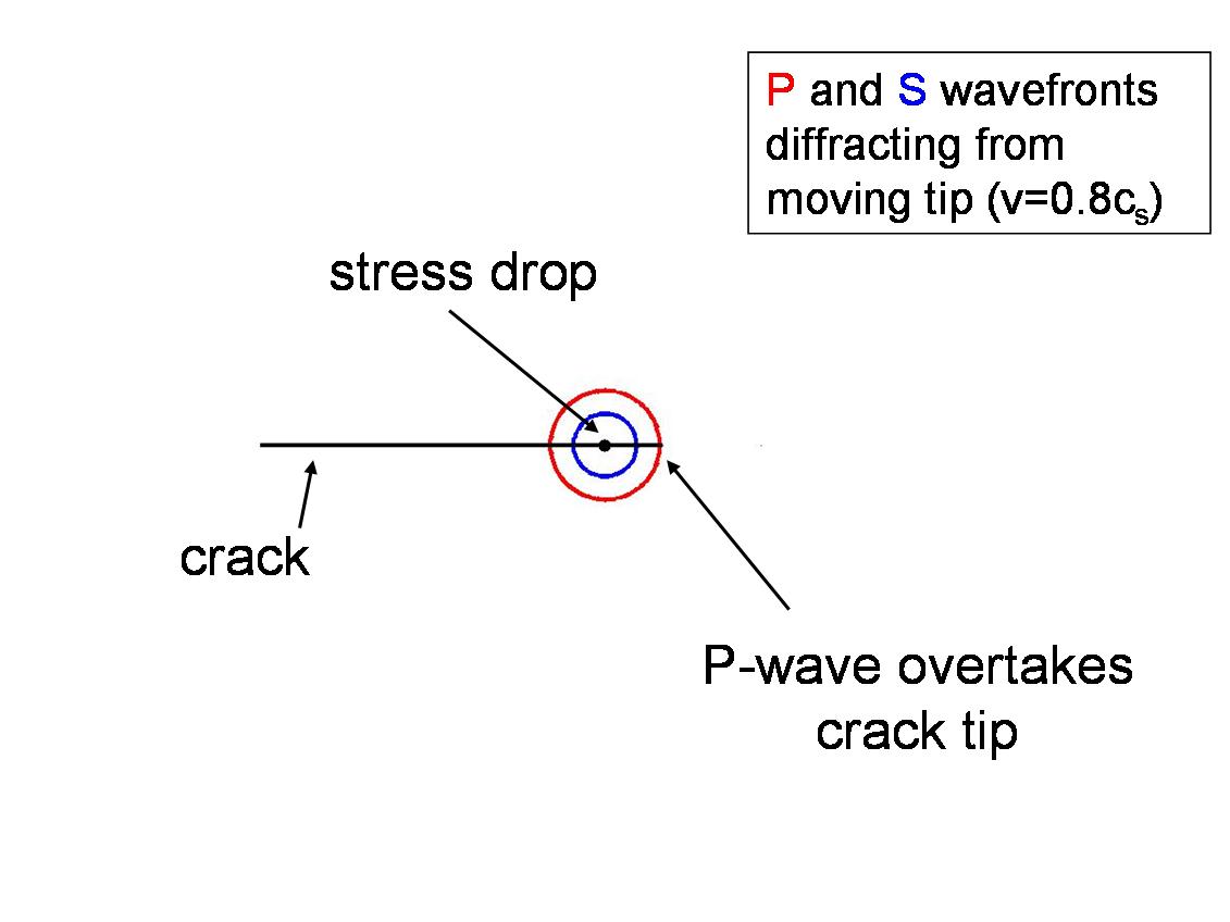
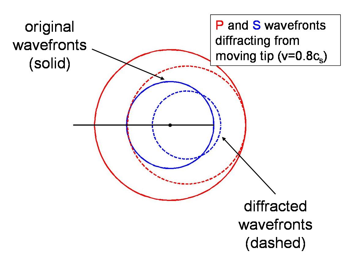
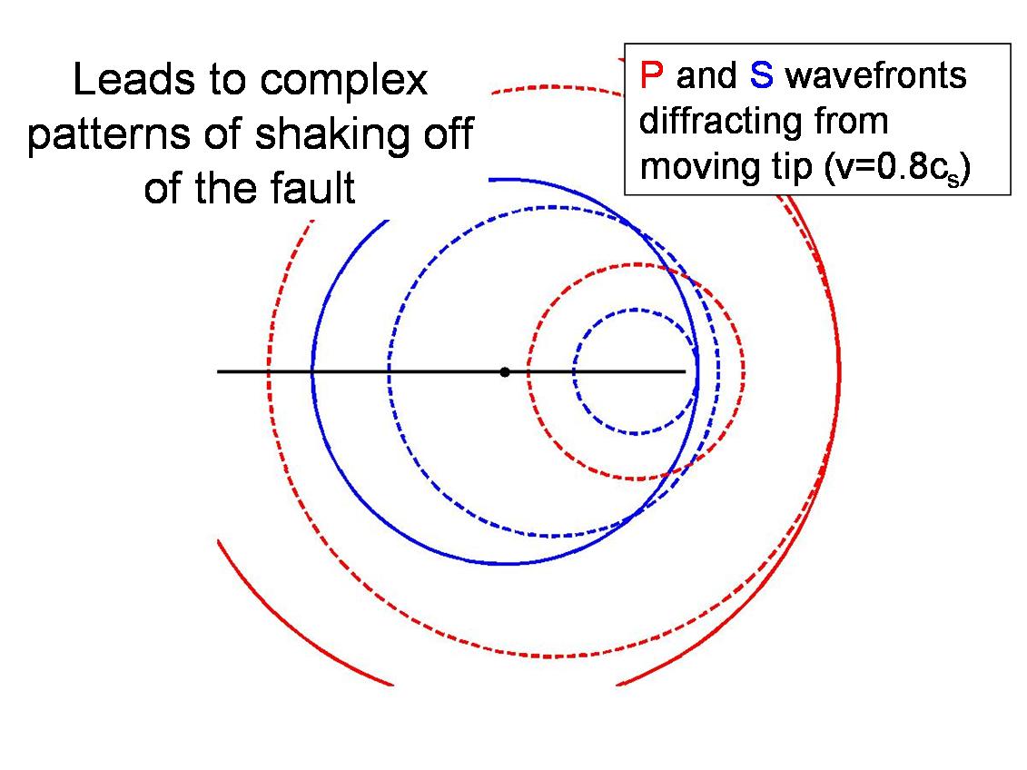
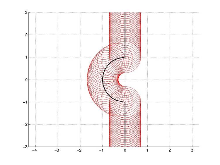
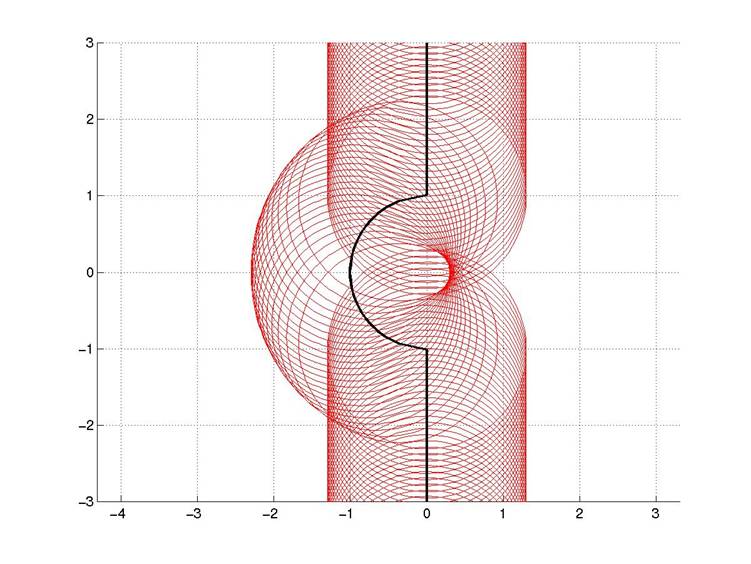
Some of these elastic waves radiate away to generate the ground shaking we experience, while others travel along the fault to the locked region ahead of the crack edge. These waves carry the shearing force to the locked section and drive it toward failure. In this way, the crack expands at a velocity comparable to the speed of elastic waves, about 4-6 km/s! That’s a good deal faster than the rate at which the plates move. As you can see, this process is cyclical, and can lead to a rapidly expanding rupture (see Figure 4).
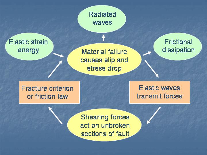
Figure 4: The dynamic rupture process. The green bubbles show the flow of energy within the system. The yellow and orange boxes show the process by which the energy conversion occurs.
Questions? E-mail Eric Dunham
Back to top
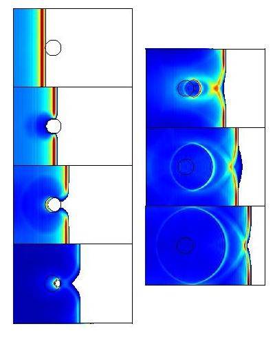
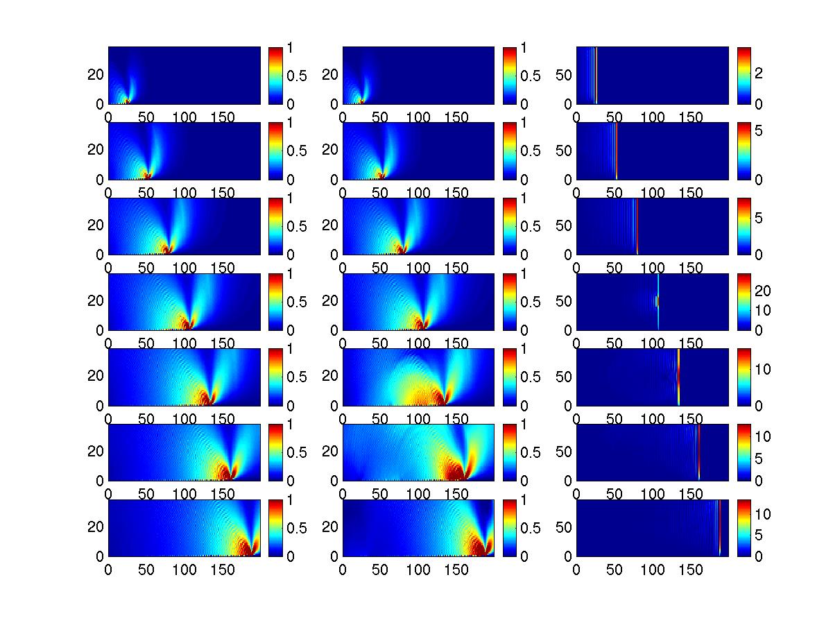
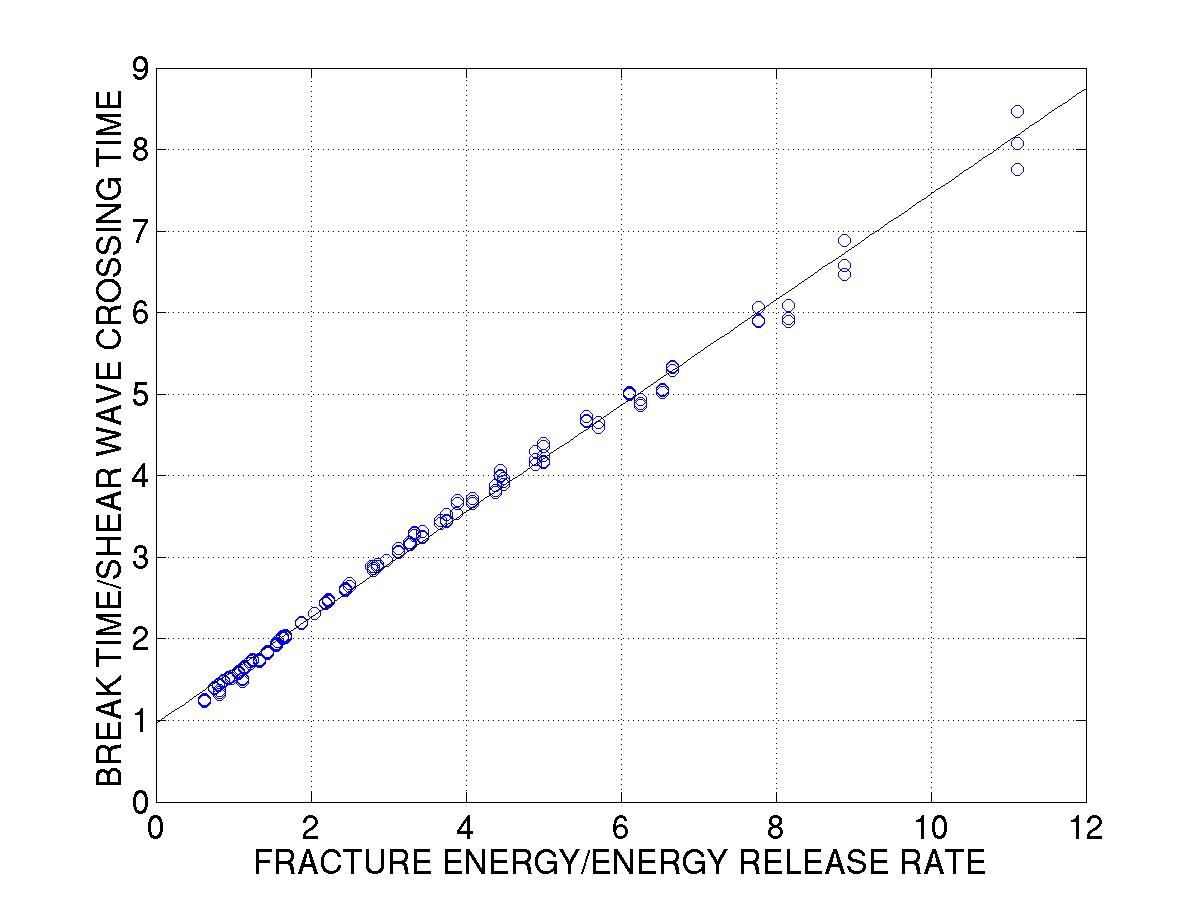
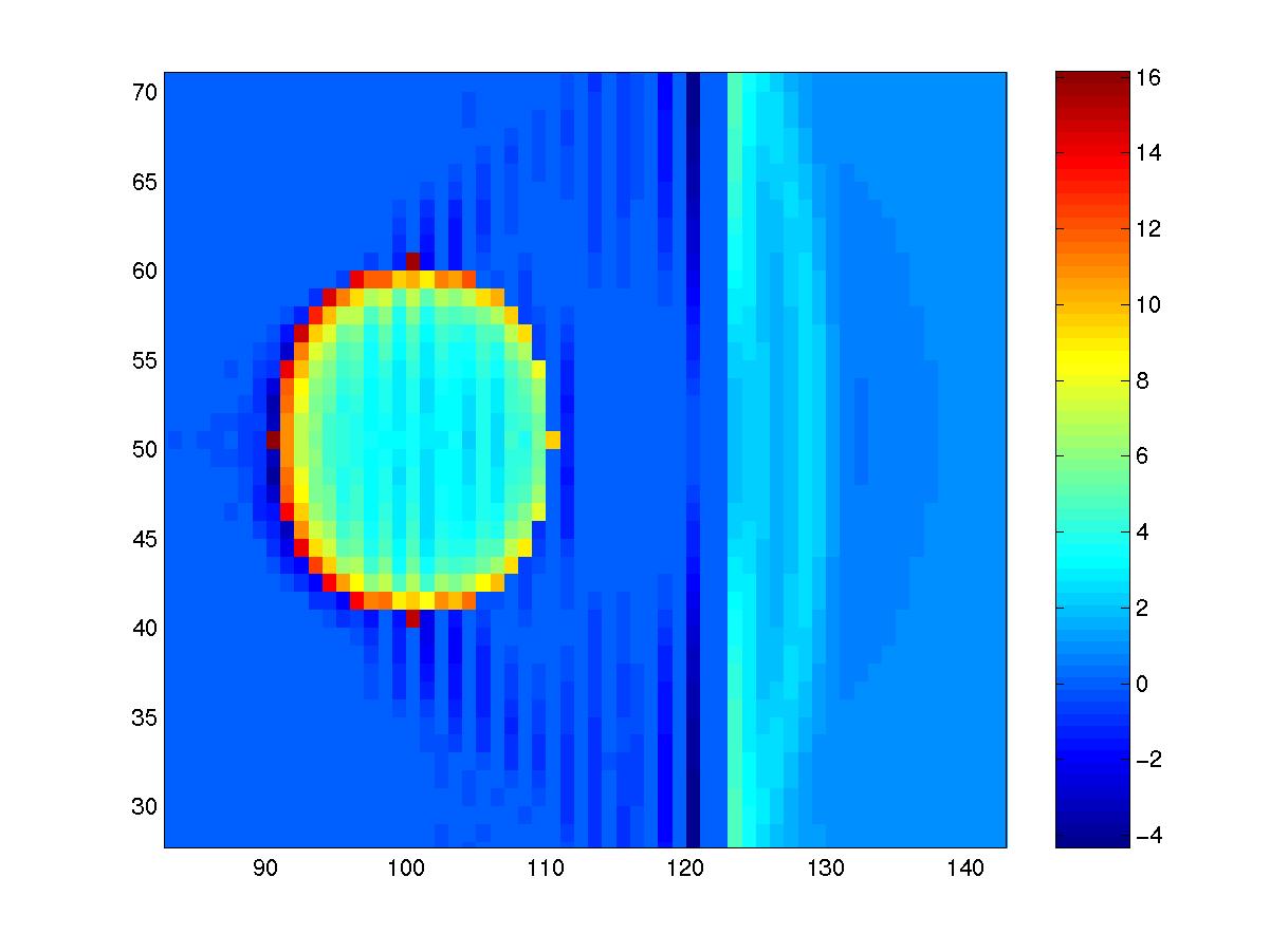
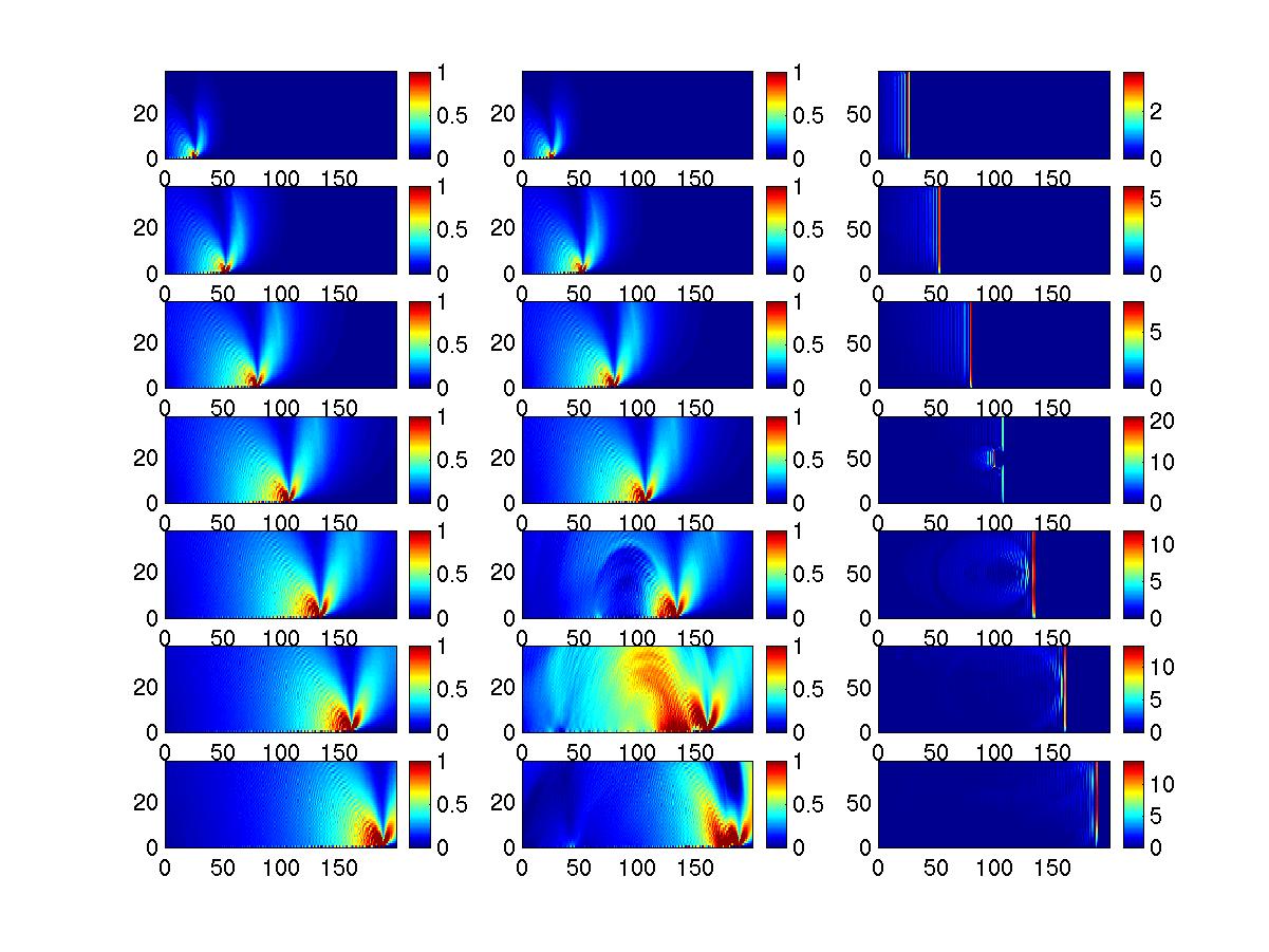
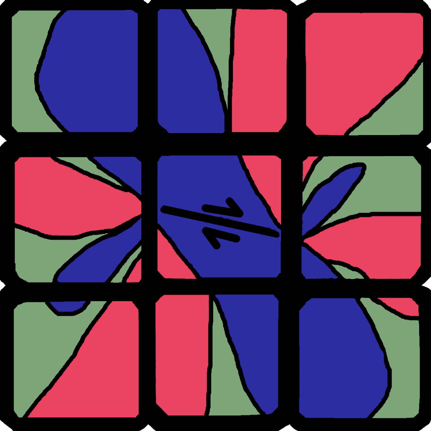
![Barrier experiments of Dunham et al. [2003]](radiation_files/barrier.gif)
![Friction Law from Andrews[1985]](radiation_files/frictionlaw.gif)