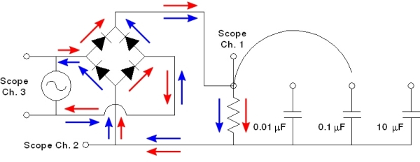
In demonstration 64.57 -- Half-wave rectifier, the positive-going half cycles of the sinusoidal output of a function generator pass through a diode and a series resistor. Demonstration 64.58 -- Full-wave rectifier, uses a center-tapped transformer and two diodes to rectify both half cycles of a sinusoid. This demonstration presents the bridge rectifier, which rectifies both half cycles of a sinusoid, and thus provides full-wave rectification, without the use of a center-tapped transformer. As we will see, while for the half-wave rectifier the output level is the peak input voltage, and for the full-wave rectifier (with center-tapped transformer) it is half the peak voltage, for the bridge rectifier the output is equal to the peak input voltage. Below is a schematic of the circuit:
Scope channel three measures the voltage across the source. Subtracting the voltage at channel two from that at channel one by means of the math function gives the voltage across the load. As in the other two rectifiers, the diodes are 1N914, and the load is 100 kilohms. (Please note: The 1N914 is NOT typically used in power rectifier circuits. It is, however, more than capable of handling the currents and voltages used in this demonstration (vide infra).) The jumper (curved wire) allows you to add any of the three capacitors to the circuit for filtering (vide infra). The red arrows show the direction of current flow during the positive half cycle, and the blue arrows show the direction of current flow during the negative half cycle. (The arrows follow the convention that current flow is in the opposite direction to electron flow.)
The bridge is arranged so that on each half cycle, the load is in series with one pair of diodes that are forward biased, while the other pair is reverse biased. The bridge therefore conducts during both half cycles, and the peak voltage across the load equals the peak voltage of each half cycle. The enlarged photograph below shows this a bit more clearly.

The peak-to-peak voltage of the input signal is 23.4 volts. One-half of this would be 11.7 volts. Because of the junction potential, as mentioned in the pages for the LED and the other rectifier demonstrations, the measured amplitude of the bottom trace is 10.6 volts, about 1.1 volts lower. This difference represents the junction potential of the two diodes that are in series with the load.
As for the other rectifiers, in order to change the rectified voltage from a pulsating DC voltage to a steady one, we can place a capacitor across the load. The capacitor charges during the positive-going portion of each half cycle, and it discharges through the load during the negative-going part. Depending on the RC time constant (see demonstrations 64.51 -- RC circuit to galvanometer and 64.54 -- RC circuit to oscilloscope), the discharge takes more or less of the time between positive half cycles, and the filtering action flattens the output voltage to a greater or lesser extent. The three photographs below show the result of adding each of the three capacitors on the circuit board:
We see that the filtering afforded by the 0.01-μf capacitor raises the tail of the half-cycle, the 0.1-μf capacitor smooths the waveform even more, leaving a large ripple, and the 10-μf capacitor takes out enough of the ripple to make the DC voltage essentially flat.
As the text for the other two rectifier demonstrations states, for a given rectifier circuit, the size of the ripple can be expressed as the “ripple factor,” r = Iac/Idc = Vac/Vdc. r also equals 1/(2√3fCRL), where f is the frequency of the ac component. As we can see from the traces above, for the bridge rectifier the frequency equals twice that of the input voltage. Since the frequency of the input is 60 Hz, the ripple frequency is 120 Hz. This expression holds only for wave forms that are approximately sinusoidal, and for loads that do not cause the output voltage to drop more than about 20% from the peak voltage. Alternatively, we can derive a simple expression for the ripple voltage. If the ripple is small, we can assume that the current through the load is constant, and from I = C(dV/dt) we have ΔV = (I/C)Δt. Δt is just the period of the ripple, so it equals 1/f, making the expression ΔV = (Iload/fC). (Here, f is double the line frequency, or 120 Hz, as mentioned above.) In doing this, we have assumed a linear discharge of the capacitor, instead of an exponential, but for constant load current, the discharge is linear. We can see from both of these expressions that for a given frequency, increasing the capacitance reduces the magnitude of the ripple, and whatever the capacitance, increasing the frequency of oscillation of the input voltage also decreases the size of the ripple. We can also see from the first two traces above that as the ripple becomes smaller, the discharge gets closer to being linear.
In this demonstration, as for the half-wave rectifier demonstration, not only can you change the value of the capacitor, as shown above, but you can also vary the frequency of the function generator to show its effect on the ripple.
As the text for the other rectifier demonstrations also states, the diodes used in a rectifier circuit must have the proper ratings so that they will not fail. The main considerations for a rectifier circuit are the maximum average forward current and the peak inverse voltage (PIV), or maximum repetitive reverse voltage (VRRM). The maximum average forward current is roughly 1/2(Vav/RL), where Vav is the average voltage and RL is the load resistance, since each pair of diodes conducts only half the time. As for the other rectifiers, if we add a capacitor to filter the output, the PIV is twice the peak voltage, since the capacitor holds the output at peak voltage while the opposite side of the bridge swings down to negative peak voltage. Because there are two diodes in series with the load, however, each diode sees only half the applied voltage, or just the peak voltage, which in our demonstration is about 11 volts. The 1N914 diodes used in this demonstration are rated for a VRRM of 100 volts and an average rectified forward current of 200 mA. While these values, especially the average forward current, make these diodes unsuitable for use in most power supply applications, they easily handle the PIV of 11 volts and average forward current of 0.11 mA present in this demonstration.
References:
1) Howard V. Malmstadt, Christie G. Enke and Stanley R. Crouch. Electronics and Instrumentation for Scientists (Menlo Park, California: The Benjamin/Cummings Publishing Company, Inc., 1981), pp. 59, 61-62.
2) Paul Horowitz and Winfield Hill. The Art of Electronics, Second Edition (New York: Cambridge University Press, 1994), pp. 45-46, 329-330.
3) Fairchild Semiconductor Corporation. Data Sheet for 1N/FDLL 914/A/B / 916/A/B / 4148 / 4448 Small Signal Diode (2002).