The square wave output of a signal generator is connected to a variable resistor and an inductor in series. The voltages across the pair (top trace), the inductor (middle trace) and the variable resistor (bottom trace) are shown on the oscilloscope, whose display you can project to the class via the data projector.
Demonstration 72.57 -- LR circuit rise time (L/R), shows the behavior of a circuit comprising an inductor and a resistor connected in series via a switch to a power supply, at the time the circuit is closed. The resistor is a light bulb, and by changing between a 40-watt bulb and a 500-watt bulb, whose resistances are greatly different, you can show that the time it takes for the current in the circuit to reach its maximum, after you close the switch, is much greater for the 500-watt light bulb than for the 40-watt light bulb. The circuit in this demonstration comprises a 100-kΩ variable resistor in series with a 10-henry inductor, placed across the output of a function generator set to produce a 200-Hz square wave. The square wave simulates a periodic connection of the free ends of the inductor-resistor pair to the output of a power supply, followed by their being shorted.
As noted in the page for demonstration 72.57, a changing magnetic flux produced by a changing current in a coil, induces an emf in the coil itself. This phenomenon is called self-induction, and the emf is called a self-induced emf. It is determined by Faraday’s Law, which states that E = -d(NΦB)/dt, where N is the number of turns in the coil. NΦB is the number of flux linkages in the coil. If the coil does not have an iron core, and it is not near any magnetic materials, NΦB is proportional to the current, i, through the coil, or NΦB = Li. The proportionality constant, L, is called the inductance of the coil. Faraday’s Law gives E = -d(NΦB)/dt = -L(di/dt). We can rewrite this as L = -E/(di/dt), from which we can see that the unit of inductance is the volt-second/ampere. The name for this unit is the henry, which is abbreviated as H.
If we rearrange the second equation above as L = NΦB/i, and then imagine a section of length l near the center of a long solenoid, we can obtain the inductance in terms of the geometrical properties of the coil. For such a section, the number of flux linkages is NΦB = (nl)(BA), where n is the number of turns per unit length, B is the magnetic field inside the solenoid, and A is the cross-sectional area of the solenoid. From Ampère’s law (by integrating around a rectangular path enclosing several turns of an ideal solenoid) we have B = μ0ni, which gives NΦB = μ0n2liA. So L = NΦB/i = μ0n2lA. Since n = N/l, L = μ0N2A/l. (μ0, the permeability constant, equals 4π × 10-7 tesla·meter/ampere, or 1.26 × 10⁻⁶ H/m. 1 tesla equals 1 N/(A·m), so 1 T·m/A = 1 N·m/A2·m = 1 N/A2. 1 H = 1 V·s/A = 1 N·m·s/(C·A) = 1 N·m/A2. So 1 H/m = 1 N/A2 = 1 T·m/A.)
If only the resistor were connected across the output of the function generator, the voltage across it would equal the output voltage of the function generator, and the current at any time would equal V/R, where V is the output voltage and R is the resistance. With the inductor in the circuit, though, as soon as current starts to flow, the self-induction in the inductor produces an emf across it. By Lenz’s Law (see demonstration 72.09 -- Lenz’s law), and as Faraday’s law above implies, this emf opposes the potential placed across it by the power supply and, thus, the rise of current through the circuit. The resistor thus experiences the sum of two opposing emfs, one from the function generator, and an opposite, time-dependent one equal to -L di/dt from the self-induction of the coil. Over time, the current increases more slowly, which causes the emf from self-induction in the coil to decrease, and the current in the circuit approaches E/R asymptotically. (The square-wave output of the function generator is, of course, time dependent, but we can choose its period and/or the size of the resistor so that this process occurs within one half cycle of the square wave.)
To find an expression for the current in the circuit, we note that the sum of the voltages across the resistor and the inductor equals the voltage applied by the function generator, or:
E = L(di/dt) + iR
The solution to this differential equation is:
i = (E/R)(1 - e-Rt/L)
which we can also write as:
i = (E/R)(1 - e-t/τL)
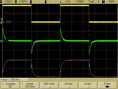
where τL, the inductive time constant, equals L/R. This is the time it takes for the current to reach 63% of its maximum value. (At t = L/R, the term in parentheses equals 1 - e-1, or 1 - 0.37 = 0.63.) The oscilloscope traces below show the operation of the circuit with the variable resistor set at three different values.
τ ≈ 0.1 ms (R ≈ 100 kΩ)
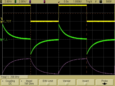
τ ≈ 0.5 ms (R ≈ 20 kΩ)
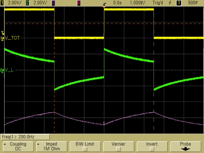
τ ≈ 2 ms (R ≈ 5 kΩ)
In each panel above, the top trace (V_TOT) shows the square wave output of the function generator, which is the voltage across the resistor and the inductor together. The middle trace (V_L) shows the voltage across the inductor, and the bottom trace (unlabeled) shows the voltage across the resistor (the difference between V_TOT and V_L). The time base for all the traces is 1.0 ms/division. For the traces in the panel at left, the variable resistor was set to its maximum value. This gives the minimum time constant we can achieve, which with the 10-H inductor is 10 H/100,000 Ω = 0.1 ms. The traces reflect an L/R time constant that is comparable to this. For the traces in the middle panel, the resistor was set to about 20 k, for a time constant of about 0.5 ms, and for the trace at the right, the resistor was set to about 5 k, for a time constant of about 2 ms.
We see that as τL becomes very small (R is very large), VL approaches zero and VR begins to resemble the input square wave, and that as the time constant becomes large compared to the length of the half cycles (R is small), VL begins to resemble the input square wave and VR decreases. (When R goes to zero, the entire voltage is across the inductor, and VL equals the input square wave.) It is interesting to compare these traces with those for the RC circuit, shown in demonstration 64.54 -- RC circuit to oscilloscope.
References:
1) Halliday, David and Resnick, Robert. Physics, Part Two, Third Edition (New York: John Wiley and Sons, 1977), pp. 720, 757, 795-9.